PE&RS August 2014 - page 700

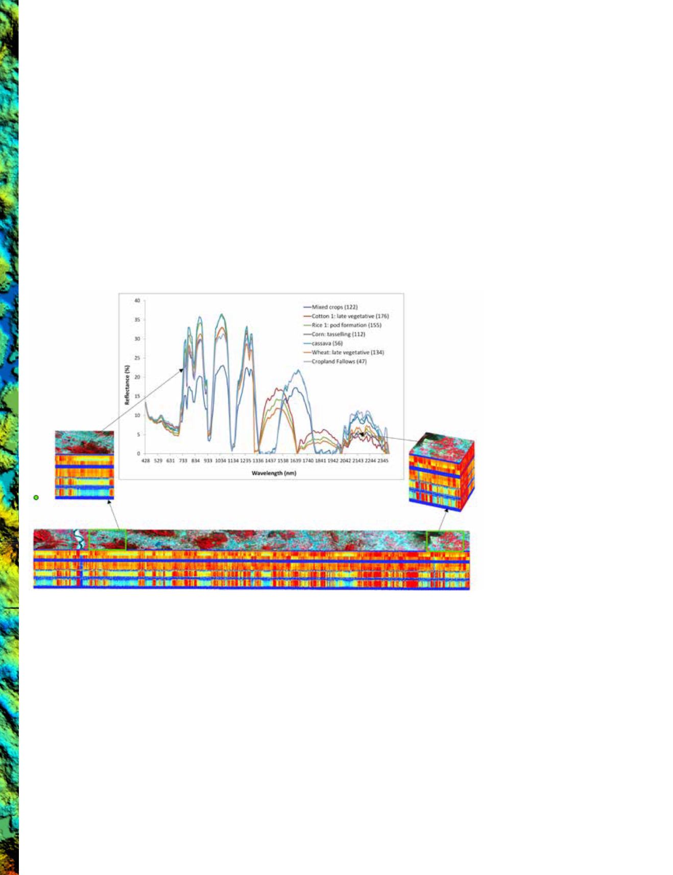
can be seen in various spectral signatures (Figure 2) there are
distinct differences between various vegetation categories or
species at specific portions of the spectrum. For example, cot-
ton, rice, and wheat crops are best discriminated using SWIR
bands (e.g., 1520 nm, 1820 nm) than anywhere in visible and
NIR bands. Similarly, others have shown (Thenkabail et al.,
2004a; Pu and Bell, 2013; Thenkabail et al., 2013) primary for-
est was most distinctive from secondary forest at wavebands
centered around 1045 nm, 1640 nm, and 2130 nm. This tells
us that hyperspectral data offers many windows of opportu-
nity to spectrally distinguish complex vegetation. However, it
requires rigorous quantitative analysis after addressing data
normalization and harmonization issues including radiometric
and atmospheric corrections (Thenkabail et al., 2004a; Pu and
Bell, 2013; Thenkabail et al., 2013), and numerous data min-
ing approaches (Bajwa and Kulkarni, 2011).
Data Redundancy and Optimal ( or
best) Hyperspectral Narrowbands
(HNBs)
The need to address large data volumes that separates real
data from noise in hyperspectral imagery cannot be over-
emphasized. Data volumes are reduced through data mining
methods such as feature selection (e.g., principal component
analysis, derivative analysis, wavelets, the lambda by lambda
correlation plots; (Thenkabail et al., 2000), and partial least
squares and vegetation indices (Mundt et al., 2006; Bajwa
and Kulkarni, 2011; Swatantran et al., 2011; Banskota et al. ,
2013; Thenkabail et al., 2013; Thorp et al., 2013; Marshall
and Thenkabail, 2014). Data mining methods lead to: (a)
reduction in data dimensionality (Bajwa and Kulkarni, 2011),
(b) reduction in data redundancy (Burger and Gowen, 2011),
and (c) extraction of unique information. However, these data
mining approaches often reduce data without identifying
which wavebands are redundant and which have unique
information content. This requires us to identify redundant
bands and separate them from valuable bands, a concept
first proposed by Thenkabail et al. (e.g., 2000) and applied by
numerous researchers later on. Often, bands that adjoin one
another (e.g., a 10 nm wide narrow bands centered at 680 nm
and a 10 nm wide narrowband centered at 690 nm) are nearly
perfectly correlated (R-square >0.99) (Thenkabail et al., 2013).
Since such bands provide similar information, it is best to
select one unique band, i.e., the band that provides maximum
information. A series of research papers by (Thenkabail et al.,
2000; Thenkabail, 2002; Thenkabail et al., 2004a; Thenkabail
et al., 2004b; Thenkabail et al., 2013) conducted rigorous
accuracy assessments (Congalton and Green, 1999; Congalton
and Green, 2008) and established that ~15 to 20 narrowbands
(e.g., Figure 3) out of 242 Hyperion HNBs provide optimal
information in classifying crops and vegetation (leaving ~220
HNBs redundant). For example, seven vegetation categories
(Figure 3), when classified using 157 calibrated, non-
atmospheric window portions of Hyperion bands, achieved
an accuracy of 92% for 15 best bands (Figure 3). Research by
Thenkabail et al. (2013, 2011, 2004, 2002) identified ~15 to
20 HNBs as optimal (e.g., Figure 3), but meta-analysis based
on a wide array of research papers consider up to 28 HNBs
(Table 2, Figure 4a) as non-redundant. Relative to HNBs,
Figure 2. Hyperspectral data cube derived from Hyperion images for an agricultural area.
“Typically,
~3 to 8 HNBs
help attain
best possible
R-square values
in modeling
agricultural
crop
biophysical and
biochemical
variables,
beyond which
the relationship
becomes
asymptotic”
700 August 2014 PHOTOGRAMMETRIC ENGINEERING & REMOTE SENSING