Compactness: 0.8) for the raw and the filtered data. Overall,
the criteria have improved values when the filtered image is
involved, indicating that the extracted segments not only have
enhanced shape, they are also fewer in number. Therefore,
the resultant meaningful objects that correspond to real
world objects can, also, ameliorate and ease the upcoming
classification rule-set implementation.
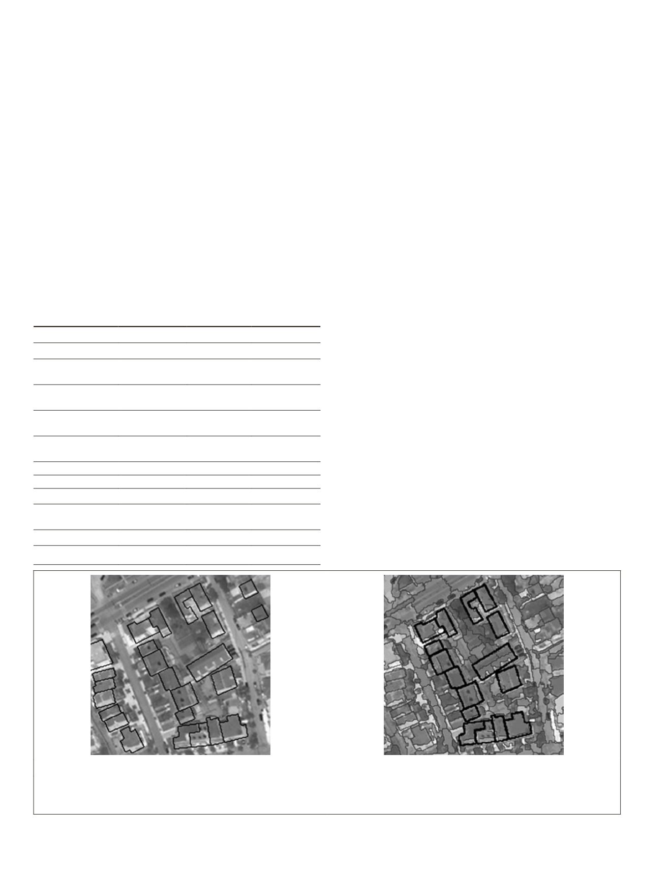
This can be, also, observed in Figure 2, where more
accurate correspondences among the reference polygons and
image objects have been settled. The filtered images produce
segments that are more close to the reference data ameliorating
the upcoming change detection classification steps.
Therefore, having the filtered image as input data, the first
segmentation level in object hierarchy is created with the
help of the existing geoinformation (buildings/roads). Under
this framework, the resulting objects correspond strictly to
the existing buildings (Figure 3a). The objects of the following
levels are based on the first object level and the multispectral
information, in a way that the new objects are bounded
by the boundaries of the existing buildings. The aim is to
generate image objects that correspond to existing buildings
and employ them for the training of the classification system.
Based on those image objects, the spectral, geometric, and
contextual features of the existing buildings are calculated
afterwards through the modeling processing (Figure 3b).
Modeling Buildings
The building model integrates knowledge about the spectral,
shape and contextual features in order to define the building
classes. The relations and the possible variations among the
urban objects have been also taken into consideration for the
definition of the adequate building extraction rules. Since the
existing geodatabase included information about the buildings
and the road network, the calculated features corresponded
to these particular land cover types. The spectral features
included the mean and standard deviation, the Normalized
Difference Vegetation Index (
NDVI
) and the Built-up Area Index
(
BAI
), which is the normalized difference of the Blue and the
Near Infrared band (
NIR
). The
BAI
was proven to be able to
identify several of the areas with asphalt and cement in the
study area and for this reason was chosen to participate in the
model (Bouziani
et al
., 2010). The shape features included the
Compactness, Length/Width, Rectangular Fit, Perimeter, Elon-
gation, Shape Index, and Relative Area and the contextual ones
referred to distances from the existing classes (Blaschke, 2010).
Definition of the Training Objects
The time difference between the image (reference date) and
the geodatabase (base date) to be updated implies changes
referring not only to newly constructed buildings, but also to
demolished buildings. Therefore, the first important step of
the learning process is to delineate those buildings that exist
in the geodatabase, but not in the image, and for this reason,
they have to be excluded from the learning process. To this
end, the proper rules have been implemented by comparing
the shape features of the objects and defining the ones that do
not belong to buildings anymore.
In particular the demolished buildings are detected
through the following process:
1. Image segmentation of the reference date based on the
vector information regarding the existing buildings in
the base date (1
st
segmentation level)
2. Image segmentation of the reference date based on the
spectral information of all the spectral bands (2
nd
seg-
mentation level).
3. Comparison of the two segmentation levels and auto-
matic identification of demolished buildings.
(a)
(b)
Figure 3. The segmentation procedure in different levels is constrained by the existing geographic information: (a) the resulted image ob-
jects in the first level (shown in black) correspond to the prior building information, and (b) the resulted image objects are the sub-objects
after the multiresolution segmentation and share the same boundaries with the existing ones (shown in bold).
T
able
1. Q
uantitative
E
valuation
T
owards
A
n
O
ptimal
I
mage
S
egmentation
;
the
R
aw
and
the
F
iltered
(S
cale
-S
pace
) I
mages
have
been
S
egmented with
the
S
ame
P
arameters
,
i
.
e
.,
S
cale
: 20, S
hape
: 0.3, C
ompactness
: 0.8
Area-based Criteria
Filtered Image Raw Image Optimal Value
Average difference
of the area [%]:
10,69
12,59
0
Average difference
of perimeter [%]:
17,64
28,83
0
Average difference
of shape index [%]:
25,32
38,57
0
Average number of
partial segments
4,82
15,94
the lowest
possible value
Fitness Function
0,17
0,22
0
Area Fit Index
0,51
0,77
0
Location-based Criteria
qLoc
6,1
6,7
the lowest
possible value
Combination of criteria
Index D
0,58
0,67
0
484
June 2015
PHOTOGRAMMETRIC ENGINEERING & REMOTE SENSING


