Table 2 reports the results of the
paired-sample
t
tests, the number
of improved tests, and the average
improved percentage. It reveals
that only
NSMA
shows improve-
ment, with
MAEs
lower than the
untransformed scheme in all study
areas (positive values in three
study areas). Paired-sample
t
tests
also illustrate that the differences
between
NSMA
and the untrans-
formed scheme are significant, as
their
p
values are less than 0.05.
Some schemes, such as
DA1
,
DA2
,
MNF
,
GLP
, and Tie3–5, have slightly
lower
MAEs
compared to the un-
transformed scheme in two study
areas but larger
MAEs
in another
study area. However, a paired-
samples
t
test cannot indicate a
significant difference, since many
of these transformed schemes have
p
values higher than 0.05.
DA1–3
,
CR
, Tie4, Tie6, and Tie7 have better
performance in only one study
area, and worse results in the other
two.
TC
,
BN
,
GHP
,
HP
, Tie1, and
DWT2
–4 have lower accuracy, as
the mean differences are negative
in all three study areas. Further,
significant differences between
the untransformed scheme and
TC
, Tie1, and
DWT2
–4 cannot be
obtained, since their
p
values are
larger than 0.05.
In addition, we counted the
number of improved tests as well
as the average improved percent-
age for each scheme. Generally,
transformed schemes (
DA2
,
DA3
,
NSMA
, Tie2, Tie4, Tie6, and Tie7)
performed better in Asheville than
in the other two study areas, as
the number of improved tests is
generally larger.
NSMA
performed
better than the untransformed
scheme in Janesville, Asheville,
and Columbus, as 67%, 69%, and
62% of the tests (respectively) have
lower
MAEs
than the untransformed
scheme. The performance of
CR
is
very unstable, with the number of
improved tests varying greatly from
11 to 32 to 87 in Janesville, Ashe-
ville, and Columbus, respectively.
In general, the improved percent-
ages in each scheme are relatively
high. Many of the transformed
schemes improved about 30%.
Discussion
Spectral variability, including
between-classes and within-class
variability, is widely present in
remotely sensed imagery. Factors
such as materials’ spectral char-
acteristics, geometry, and other
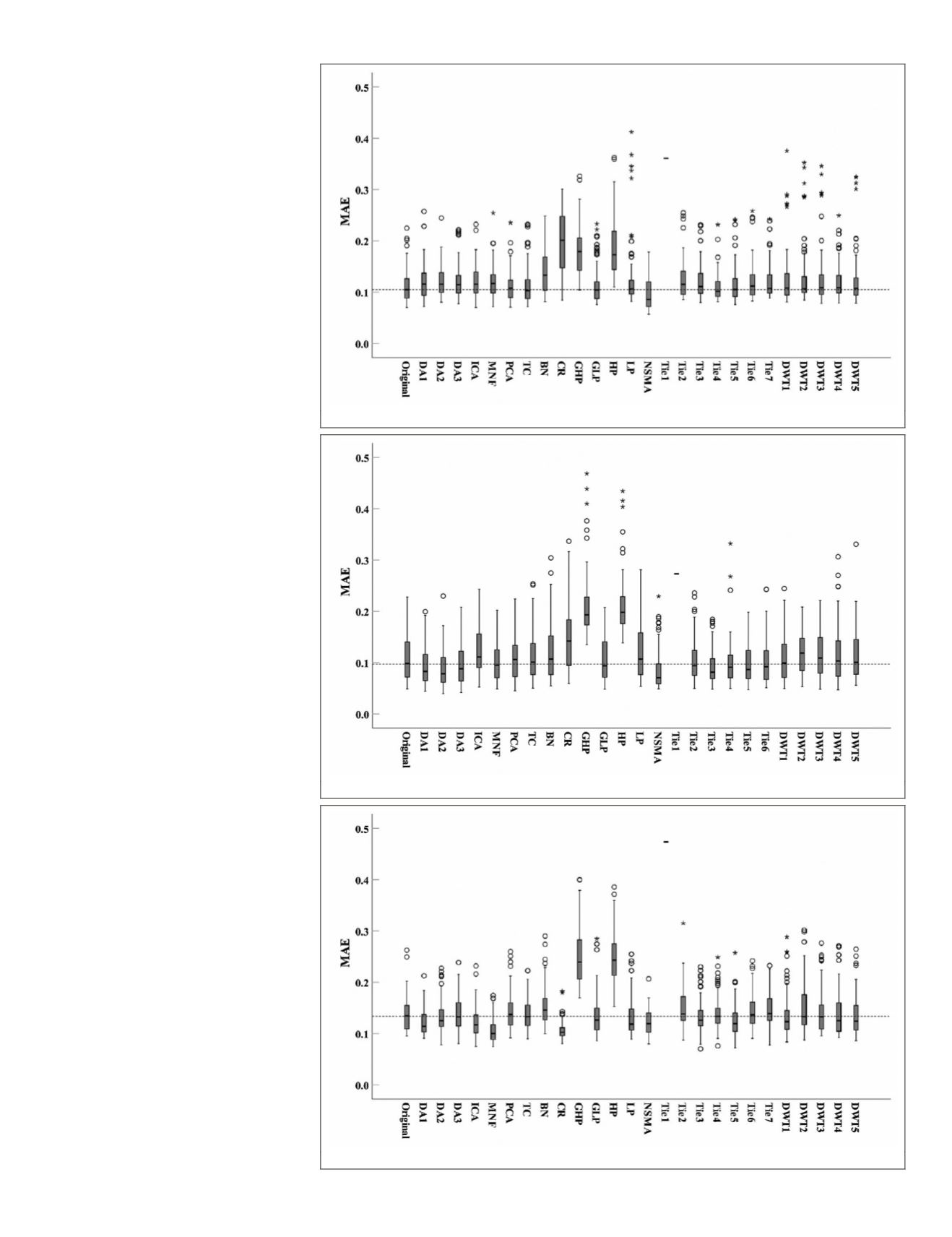
Figure 2. Box plot of mean absolute error in Janesville, Wis., United States.
Figure 3. Box plot of mean absolute error in Asheville, N.C., United States.
Figure 4. Box plot of mean absolute error in Columbus, Ohio, United States.
PHOTOGRAMMETRIC ENGINEERING & REMOTE SENSING
July 2019
525


