PE&RS January 2016 - page 66

as inputs, which helps improve the performance since the
operations can be executed in memory. Specifically, the script
uses a series of nested “Con” conditional statements from the
Spatial Analyst toolset. The Con function evaluates a condi-
tion on a per-pixel basis, and can either output a raster value
or initiate another Con statement nested within it.
Accuracy Assessment
An accuracy assessment was conducted on both the LULC and
impervious surface maps independently. A set of 300 random
testing samples was created for each classification map. This
yielded an average of 50 samples for each land-cover class,
which is the minimum number of samples that is required to
represent which classes are being confused in the matrix (Con-
galton and Green, 2009). Each sample represents one single
pure pixel. This sampling strategy was the same as that was
used by Yuan (2010) who classified the 2006 LULC based on
Landsat imagery in TCMA and assessed the classification accu-
racy using 300 randomly located sample units. Because of the
retrospective nature of our study, the testing samples could
not be collected in the field. Instead, they were obtained based
on visual interpretation of the 1 m resolution NAIP imagery
itself. Typically, fewer mixed pixels are present in high-resolu-
tion remote sensing imagery; however, the problem still exists
(Wu and Yuan, 2011). For example, Wu (2009) found that the
4 m resolution Ikonos imagery contained 40 to 50 percent of
mixed urban pixels for Grafton, Wisconsin. Therefore, in this
study, a single pixel was used as the sampling unit in order to
minimize samples with mixed land covers. Further, the use of
pixels for accuracy assessment can avoid many of the compli-
cations that arise when other spatial units, such as blocks of
pixels or polygons, are used (Stehman and Wickham, 2011;
Wickham et al., 2013). In addition, the pixel was replaced
with another randomly added one if the cover type identifica-
tion was questionable. For example, sometimes it was difficult
to differentiate cropland from other vegetated areas based on
the visual interpretation. Nevertheless, only very few pixel
samples out of the 300 total were replaced. Figure 3 displays
the locations of the 300 sample units. Because bare soil (<2
percent) and water (<6 percent) are rare in the study area, the
sample sizes for them were much less than 50, but they were
still represented by the randomly distributed samples.
Error matrices were generated consequently for both maps,
with the columns and rows representing the reference data
and the classified values, respectively (Congalton, 1991). The
overall accuracy, per-class user’s and producer’s accuracies,
and Kappa statistic were also calculated. Producer’s accuracy
indicates how well a certain area can be classified, while
user’s accuracy reveals the probability that a pixel classified
on the image actually represents that land-cover category on
the ground (Story and Congalton, 1986; Congalton and Green,
2009). The Kappa statistic proposed by Congalton and Mead
(1983) measures how well the classification agrees with the
reference data after removing the proportion of agreement that
could be expected to occur by chance.
Results
Classification Results
The final 1 m LULC classification map is shown in Plate 1a.
As the larger-scale maps show, detailed land-cover features,
such as small water bodies, residential dwelling units, and
local streets can be identified in this high-resolution classifi-
cation map. The other vegetation was classified as the largest
land-cover class with 2,943 km2, or 38.2 percent of the TCMA.
This was followed by forest (1,999 km2; 26 percent), cropland
(1,366 km2; 17.7 percent), urban (867 km2, 11.3 percent), wa-
ter (439 km2; 5.7 percent) and bare soil (90 km2, 1.1 percent).
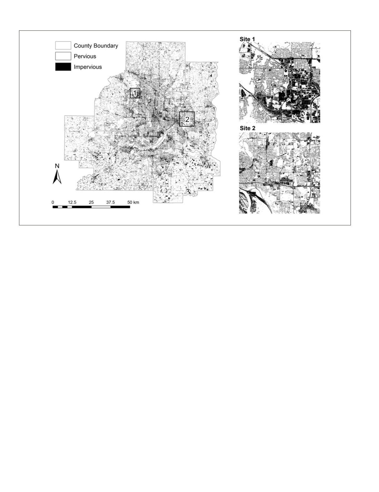
The classified impervious surfaces based on the decision
tree method are similar to those of urban and bare soil land-
cover from the object-based classification, which is expected
since urban surfaces and compacted soil is the main constitu-
ent of impervious surfaces (Figure 4). The total impervious
Figure 4. One-meter resolution impervious surface classification map of TCMA.
66 January 2016 PHOTOGRAMMETRIC ENGINEERING & REMOTE SENSING