percentage of observations that fell within the prediction inter-
val for each integer value covering the range in predicted values.
Prediction Error from Linear Regression
To develop context for our approach, we also examined the
behavior of prediction error based on multiple regression. The
purpose for this is so readers can compare the behavior of our
approach to prediction to that of multiple regression. Devia-
tions in the results between our approach for random forest
and the multiple regression approach helps to identify areas
were our approach could be improved.
Using the sample data (500 observations), we parameterized
linear regression models for
y
1
,
y
2
, and
y
3
. The model form
was
y
=
X
∙
β
+
ε
. We predicted values and 95 percent prediction
intervals for Y
1
(the Normal High population), Y
2
(Normal Low
population), and Y
3
(Model Misspecification population) based
on standard equations (see Draper and Smith, 1981 for back-
ground). For each population we also examined the percentage
of observations that fell within the prediction interval for each
integer value covering the range of predicted values.
Case Example Using Real (Unsimulated) Data from Georgia
We provide a case example for percent tree canopy cover map-
ping based on data from Coulston
et al
. (2012) for Georgia. The
dependent variable was percent tree canopy cover estimated
by photo interpretation of 2009 National Agriculture Imagery
Program (
NAIP
) photography for approximately 4,160 sample
locations. The independent variables were based on leaf-on
Landsat-5
TM
imagery from 2008 to 2009 and elevation data.
The six reflective Landsat-5
TM
bands, normalized difference
vegetation index, and tasseled cap were also used. Slope and
cosine of aspect were derived from the elevation data and also
used as predictor variables. Based on these data, we fit a ran-
dom forest model which had a pseudo-R
2
(Liaw and Wiener,
2002) of 0.85 (
RMSE
= 13.2) and created a predicted surface of
percent tree canopy cover (example area in Plate 1). We note
that there is a substantial amount of area where, based on the
NAIP
imagery, there were no trees and hence the percent tree
canopy cover should be zero. Many of these areas have pre-
dicted values in the 0.5 to 10 percent range. Our goal is to use
the previously described Monte Carlo technique to mask out
areas where the 95 percent prediction interval includes zero.
To implement our Monte Carlo procedure for this problem,
note that we are interested in the uncertainty when the true
value is zero and the predicted value is >0. In this specific sit-
uation we want to estimate the value of
τ
ˆ
such that 95 percent
of the true zero values are within
τ
ˆ
·
sd
(y
ˆ
) percent of zero. The
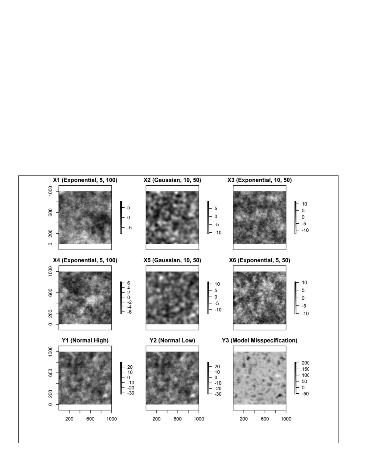
Figure 2. Simulated independent (X) and dependent (Y) variables. For the independent variables the variogram model, the variance
parameter, and the scale parameter are denoted in parentheses. For background on variogram models see Isaaks and Srivastava (1989)
for an example.
192
March 2016
PHOTOGRAMMETRIC ENGINEERING & REMOTE SENSING


