requirements this fact will be reflected in their metadata (re-
member the sentence “This map complies with
NMAS
”). But a
sampling plan establishes and makes explicit to both producer
and acquirer (user) clearer than a
PAAM
the conditions of the
process: definition of lot, lot size, sampling method, sample
size, and producer’s and user’s risk (described below), etc.
The decision from an investigated sample on whether
or not a lot satisfies stated requirements can be carried out
through hypothesis testing (achieving a pass/fail decision).
A statistical hypothesis is a statement about a probability
distribution function or about the values of the parameters
of a probability distribution function (parametric case). In
statistical testing two alternatives are always considered: (a)
H
0
: the so-called Null Hypothesis, and (b) H
1
: the so-called
Alternative Hypothesis. For example, in relation to
PAAM
s, the
EMAS
applies two tests together (bias tests and variance tests)
to each positional coordinate (X, Y, and Z).
Since sampling is a random procedure, two kinds of errors
may be committed. If the
H
0
is rejected when it is true, then a
type I error (
α
) has occurred. If the
H
0
is not rejected when it is
false, then a type II error (
β
) has occurred. The Type I error is
called producer’s risk because it denotes the probability that
a good lot/product will be rejected, or the probability that a
process producing acceptable values of a particular quality
characteristic will be rejected as producing unsatisfactory
ones. The Type II error is called user’s risk because it denotes
the probability of accepting a lot/product of poor quality.
Sometimes it is more convenient to work with the power of
the test (Montgomery, 2001), which is the probability of cor-
rectly rejecting
H
0
(Power = – β = P{reject H
0
}).
In relation to the size
n
of the sample when testing statisti-
cal hypotheses, the general procedure is to specify a value for
α
and then to design a test procedure so that a small value of
β
is obtained. Thus the producer’s risk is directly controlled
or chosen by
α
;
and the user’s risk is generally a function of
n
and is controlled indirectly. The larger the size of the sample,
the smaller the user’s risk (Montgomery, 2001). In general,
PAAM
s provide a sample size in an attempt to ensure the pro-
ducer risk (remember the sentence “at least 20 points”). This
suggested sample size is not related to the size and variability
of the population and does not ensure that user risk will be
kept under a specific threshold. Only recent proposals, such as
the new
ASPRS
positional accuracy standard (
ASPRS
, 2015), re-
late the required sample size to the size of the project area. In
ISO
2859 the size
n
is related to lot size and established risks.
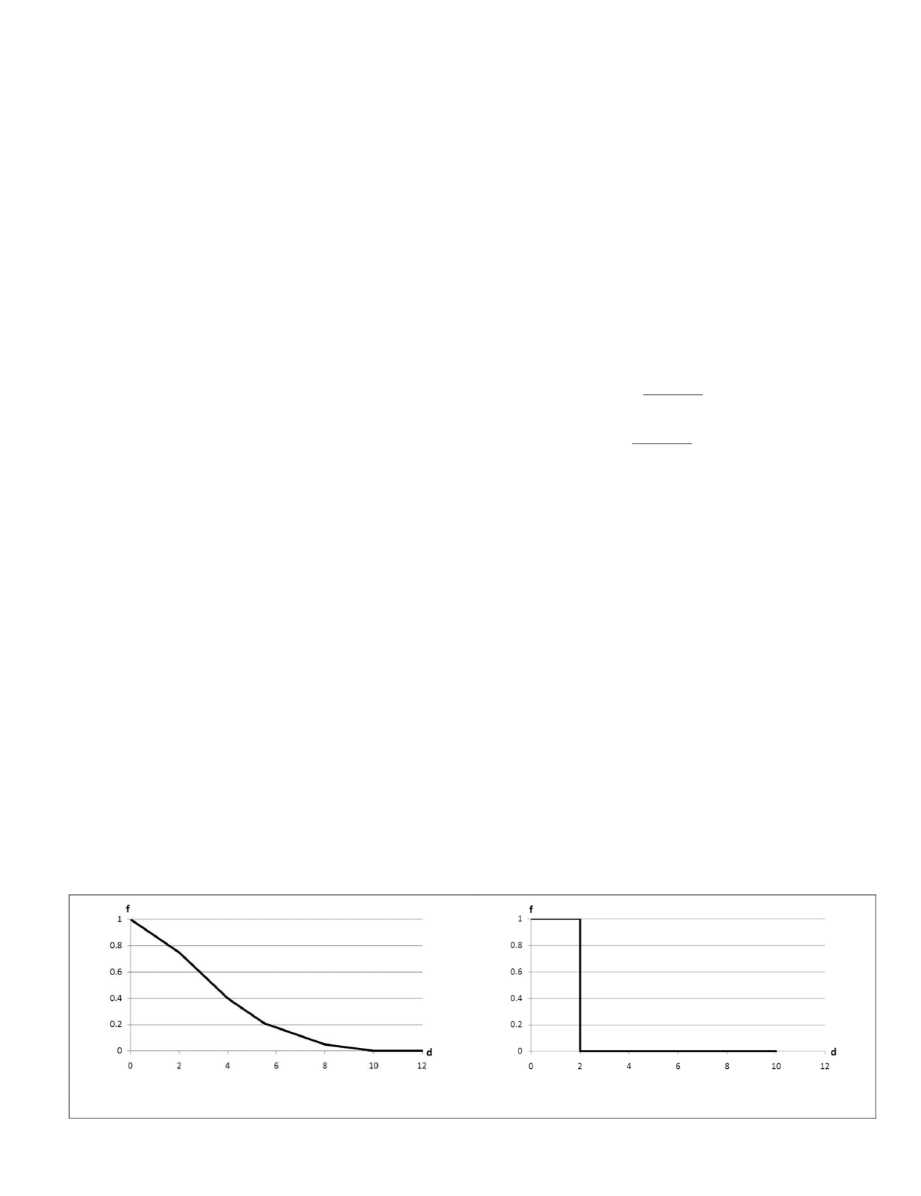
Acceptance plans are summarized by means of Operating
Characteristic curves (
OC
curves) (Figure 1).
OC
curves plot
the probability or frequency
f
of accepting lots in the Y-axis
versus the percent defectives
π
d
on the X-axis. When it comes
to 100 percent control
OC
curves represent an ideal case and
have a step shape (Figure 1a). Good lots are always accepted,
and bad lots are always rejected. Because of the sampling
randomness, actual
OC
curves are not step-shaped (Figure 1b).
Thus, an important feature of a sampling plan is how it dis-
criminates between lots of high and low quality. The ability of
a sampling plan to discriminate between lots of high and low
quality is described by its
OC
curve. A sampling plan cannot
provide perfect discrimination between good and bad lots be-
cause of the randomness of the sampling, so some low-quality
lots will inevitably be accepted and some high-quality lots
will inevitably be rejected. The degree to which a sampling
plan discriminates between good and bad lots is a function of
the steepness of its
OC
curve: the steeper the curve, the more
discriminating the sampling plan.
A common approach to the design of an acceptance sam-
pling plan is to require that the
OC
curve pass through two
designed points (Montgomery, 2001). Usually the two points
used are those corresponding to the user and producer risks.
Assuming that a binomial approximation is appropriate, the
sample size
n
and the acceptance number
c
are the solution to
the equations Equation 1 and Equation 2:
1
1
0
1
1
− =
−
(
)
−
=
−
∑
α
d
c
d
n d
n
d n d
p p
!
!
!
(
)
(1)
β
=
−
(
)
−
=
−
∑
d
c
d
n d
n
d n d
p p
0
2
2
1
!
!
!
(
)
(2)
where
α
is the Size of Type I error (producer’s risk),
β
is the
Size of Type II error (user’s risk),
n
is the Sampling size,
c
is the Acceptance number,
d
is the
Number of defectives in the sample,
p
1
is the Probability of producer risk for the point, and
p
2
is
the Probability of user risk for the point.
Equation 1 and Equation 2 are nonlinear and there is no
simple direct solution. Duncan (1986) gives a description of
some techniques for solving this system of equations: the Lar-
son binomial nomograph can be used as a graphical approach
and Kapusta
et al
. (2011) propose a mathematical model for de-
signing specific acceptance plans and provide a Matlab
®
code.
ISO 2859-1 and ISO 2859-2
ISO 2859-1
Acceptance sampling was first introduced during World War
II to determine whether to accept or reject a given batch of
military supplies. A cost (and time) saving method was needed
which would not require 100 percent of elements to be tested,
while still maintaining an adequate quality level. Dodge (1969)
identifies July 1942 as the birth of this standard under the title
of
Standard Inspection Procedures
. It achieved the status of De-
partment of Defense Standard,
JAN-STD-
105, with the develop-
ment by the Statistical Research Group of Columbia University
(a)
(b)
Figure 1. An operating characteristic curve: (a) operating curve for an ideal situation, and (b) operating curve for a sampling situation.
PHOTOGRAMMETRIC ENGINEERING & REMOTE SENSING
August 2015
659


