developed on the population, not on a parameter of the popu-
lation. This idea is illustrated in Figure 5.
The
BaM
represents the error behavior in the population,
so given a metric tolerance
Tol
(here being the maximum po-
sitional error in meters one is willing to accept), the percent-
age of error cases greater than the desired
Tol
is
π
. In other
words,
Tol
is the value corresponding to the
1-
π
percentile. In
a control sample of size
n
, the fact that the error
E
i
in element
i
verifies
E
i
>Tol
is defined as a fail event in a binomial sense
(we call it a “positional defective: in this case). The
BiM
con-
sists of counting the number of positional defectives,
f
. This
test follows a Binomial
B(n,
π
)
distribution, and the probabil-
ity of positional defectives is:
P F f F B n
n
k
k f
n
k
n k
≥ →
( )
=
−
(
)
=
−
∑
,
π
π
π
1
(3)
where
π
=
P
[
E
i
>Tol
] is the probability (
BaM
model) that a
point
i
has an error value,
E
i
, greater than the specified toler-
ance,
Tol
;
F
is the random variable “number of defective
points in a sample of size
n
”;
f
is the number of sampling
points that are defective (that is to say, their ECM is greater
than
Tol
;
n
is the sampling size;
k
is a summation index (we
sum all probabilities between
k
=
w
and
k
=
n
;
P
[
A
≥
b
|
A
(
θ
)]
is the operator “probability”– that is to say, it indicates the
value of the probability that the random variable
A
takes a
value greater than or equal to
b
when the random variable
A
follows a probability distribution
with parameter
θ
; and
B
(
n,
π
) is the binomial distribution with parameters
n
and
π
.
The null hypothesis is:
H0: The
SDS
is adequate. Given a signification value (
α
) (type
I error or producer’s risk), it means that errors are distributed
according to the
BaM
and only
π
percent of cases are greater
than
Tol
versus
H1: The
SDS
is not adequate.
Now the question is how to use this model in conjunction
with
ISO
2859-1. The answer is relatively easy because this
method is based on counting fail events (we call them here
“positional defectives”) and counting of defectives/defects
is what we need in order to apply
ISO
2859-1. Given a ran-
dom sample taken from a lot, the idea is to consider that an
element is of good quality if its error is less than the toler-
ance and that an element is a positional defective if its error
is greater than the tolerance. But some additional explana-
tions are needed. In positional controls, we are accustomed
to working with root mean squared errors or with standard
deviations and with confidence intervals in order to express
the positional accuracy of a data set. But in
ISO
2859-1 we
must use another parameter in order to express the quality of
a lot, the previously defined
AQL
. The preferences of the user
are now expressed by the pair
{Tol,
AQL
}
: the desired metric
Tol
and the upper limit of the percentage of cases that are
greater than this tolerance and which he is willing to tolerate
in accepted lots.
Nevertheless, there is a relation between both
Tol
and
AQL
and this relation comes from the
BaM
. The relation is that
AQL
=f(
π
)
, where
π
is the same as previously defined. Looking
at the
AQL
values (…0.65 % , 1 % , 1.5 % , 2.5 % ...) proposed
in
ISO
2859-1, it is clear that the tolerance must be situated
on the right side of the
BaM
model and it must be selected in
order to allow only small percentages of positional defectives.
For the producer to obtain a high acceptance of his lots, he
must work with processes that, for the same
Tol
, ensure that
the actual defective percentage is less than the
AQL
. This can
be stated in another way: given a
BaM
and a tolerance value
Tol
, the
AQL
value should be chosen to be greater than
π
. This
explanation has been developed considering that
AQL
and
π
are subrogates of
Tol
, but the same is also valid if
Tol
is con-
sidered a subrogate of
AQL
and
π
.
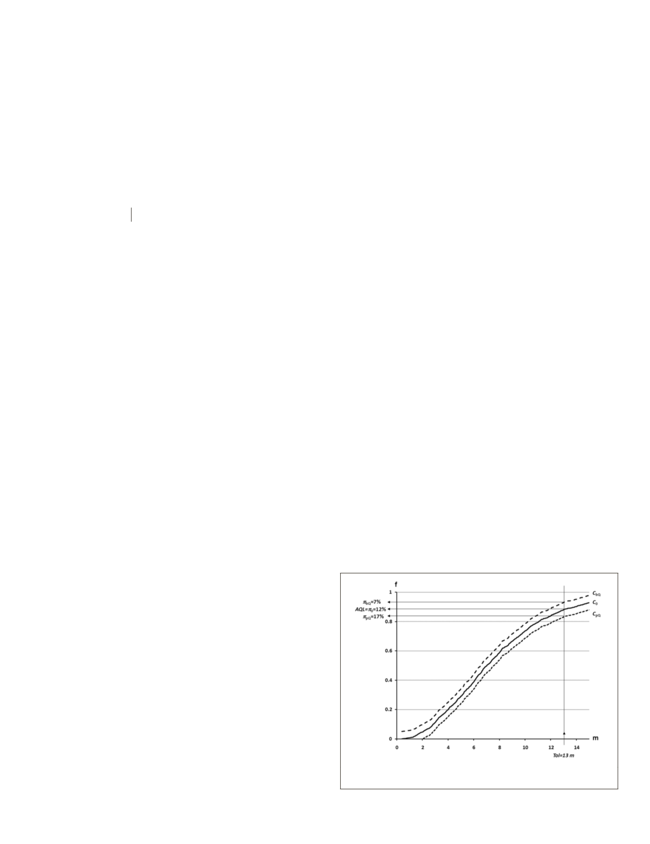
Figure 6 shows these ideas graphically. Let us consider a
BaM
represented by the solid curve labeled with
C
o
; if
Tol =
13 m through the
BaM
we obtain that
π
o
=
12 percent
,
meaning
that 12 percent of position errors are greater than 13 m. If we
want
AQL
to =
π
o
=
12 percent , it means that in order to assure
a high average of accepted lots, the producer must be able to
supply data with some better positional quality, which means
that the actual
BaM
of the product must be a curve over the
C
o
; for example, the curve labeled with
C
bQ
. Because
π
bQ
=
7
percent
<
π
o
=
12 percent, this situation assures a high level of
acceptance. But if the data supply is of a poorer quality than
demanded, the situation can be shown graphically by the
curve labeled
C
pQ
. Because
π
pQ
=
17 percent
>
π
o
=
12 percent
this situation assures rejections and the stopping of the sup-
ply by means of applying
ISO
2859-1 switching rules.
The above example is based on an empirical
BaM
(observed),
but we can also work with parametric models. For example,
for a specification of a positional error of 1 m in each coordi-
nate (planimetric error of 2.4477 m for 95 percent confidence),
we have
Tol
= 2.4477 m and
π
= 5 percent, so the
AQL
should
be slightly higher than 5 percent; and it means using tabulated
values of
ISO
2859-1 that
AQL
= 6.5 percent, so that in this case,
the control specification is (
Tol
= 2.4477 m,
AQL
= 6.5 percent).
Also, the presence of bias and outliers is related to the
AQL
by means of the
BaM
. The situation is very simple; in the case
of bias there is a right shift of the entire
BaM
. This means that:
• For the same initial Tol, the
π
value increases dramati-
cally and as a consequence
AQL
increases.
• For a given
AQL
the Tol must be increased.
In the case of outliers, there is down shift of the right tail
of the
BaM
. This right tail is the part of the model that accu-
mulates frequency coming from the largest error values. This
down shift of the right tail is equivalent to a partial right shift
of the base model. In this case we must pay attention to the
position of the
Tol
with respect to the right tail of the model
affected by the outliers. If the
Tol
is not in the affected tail,
the situation is similar to the prior one; but if the
Tol
is in the
affected tail, the situation is totally equivalent to a general
shift of the base model by bias.
It is relevant to note that the presented method is also valid
when the
BaM
is unknown. By taking the user’s preferred values
{Tol,
AQL
}
and by counting the positional defectives in the
sample, this procedure can be applied protecting the user com-
pletely. Here the problem is for the producer if the actual
BaM
of
Figure 6. Relations between metric tolerance (
Tol
), AQL and π in a
Base Model.
PHOTOGRAMMETRIC ENGINEERING & REMOTE SENSING
August 2015
663


