p
v
v
v
=
+
+…+
=
=
=
∑ ∑
∑
λ
λ
λ
λ
λ
λ
1
1
1
2
1
2
1
i
n
i
i
n
i
n
i
n
i
n
(10)
p
v
=
=
=
∑ ∑
1
1
1
i
n
i i
n
i i
λ
λ
(11)
In above equations,
λ
i
and
v
i
(
i
= 1,2,…,
n
) are the eigenvalues
and eigenvectors of
S
w
–1
S
b
, respectively.
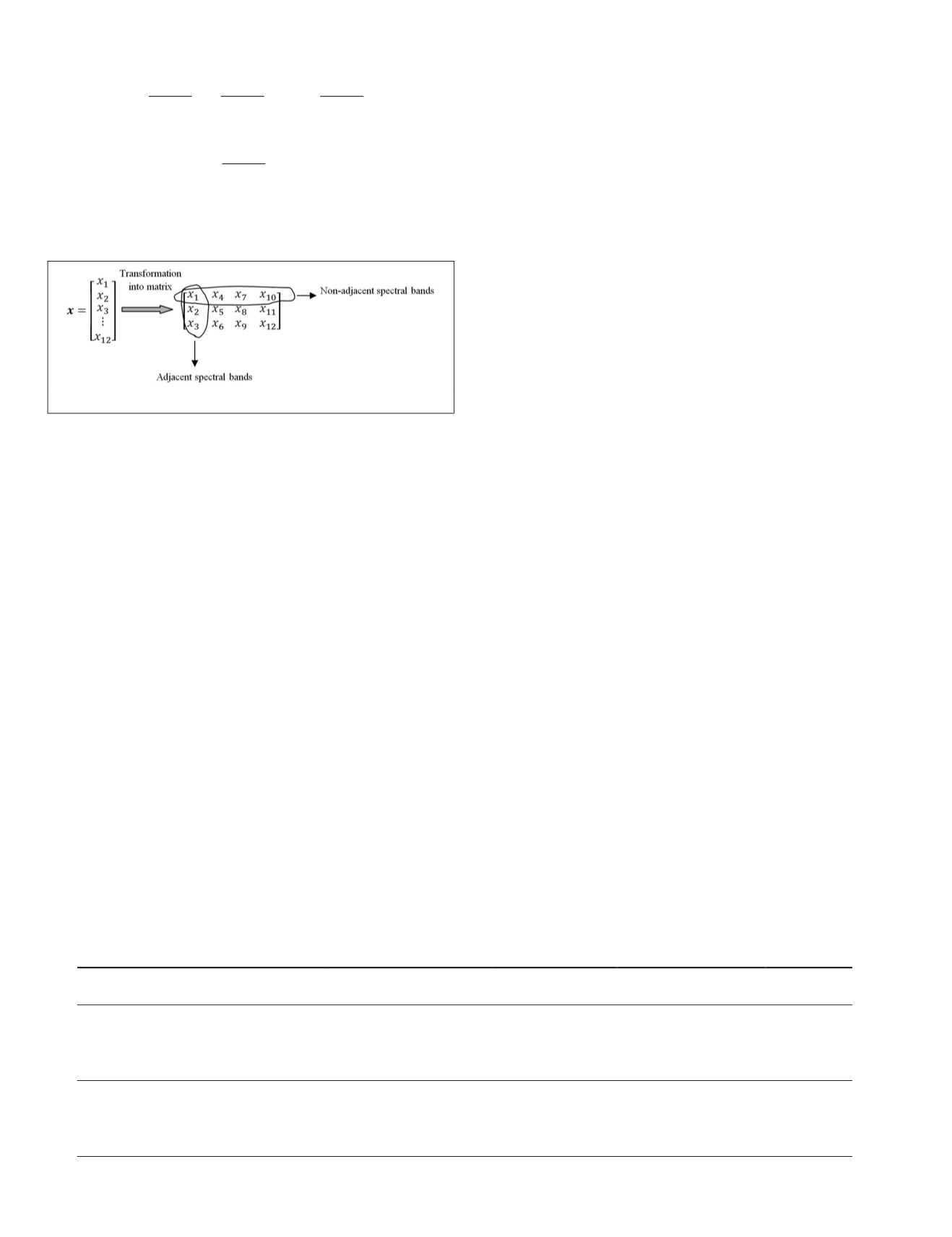
Figure 1. How to arrange features in the matrix form.
The transformation of a feature vector of each pixel of hy-
perspectral data into a feature matrix and how to arrange fea-
tures in the matrix form is shown in Figure 1. In this figure,
d
= 12,
m
= 3, and
n
= 4. As seen from this figure, each column
of feature matrix contains
adjacent spectral bands. Thus, it
may contain redundant information while each row of feature
matrix contains non-adjacent spectral bands. Therefore, the
rows contain more useful spectral information than columns.
Based on the aforementioned reasons, we can calculate the
scatter matrices using alternative way as follows:
S
b
=
i
n
c
=
∑
1
n
ti
(
A
–
i
–
A
–
)
T
(
A
–
i
–
A
–
)
T
(12)
S
w
=
i
n
c
=
∑
1
j
n
ti
=
∑
1
n
ti
(
A
–
ji
–
A
–
i
)
T
(
A
–
ji
–
A
–
i
)
T
(13)
The use of Equations 12 and 13 for calculation of scatter
matrices in the
2DLDA
approach notably improves the classi-
fication accuracy in comparison with scatter matrices calcu-
lated by Equations 5 and 6. As a result, this improvement for
the Indian dataset is on average 30 percent, and for the Pavia
dataset is on average 19 percent.
S
b
and
S
w
obtained by Equa-
tions 12 and 13 are
m
×
m
matrices. In this case, the number
of extracted features is equal to
n
where
n
is the number of
columns of matrix
A
. In this case, for extracting
n
features
from the original feature vector (
x
d
×1
), we select
ε
so that
d
+
ε
becomes divisible by
n
. To deal more with the singularity of
S
w
and to improve the classification accuracy, we regularize
the
S
w
as follows (Kuo and Landgrebe, 2004):
S
w
= 0.5
S
w
+ 0.5
diag
(
S
w
).
(14)
The comparison of two formulas for calculation of scatter ma-
trices in the proposed
2DLDA
approach is shown in Table 1.
Experimental Results and Discussion
In this section, we evaluate the performance of the proposed
method compared to some popular feature extraction methods
such as
LDA
,
GDA
, and
NWFE
. Four real hyperspectral datasets
are used for doing experiments. The Indian Pines scene was
collected over Northwestern Indiana in June of 1992 by the
Airborne Visible/Infrared Imaging Spectrometer (
AVIRIS
) (Green
et al.
, 1998). This scene contains 145
×
145 pixels, and has 16
classes in the agricultural/forest area in which a subset of 10
classes was selected for our experiments. This image com-
prises 224 spectral bands which it was initially reduced to 200
by removing strong water vapor bands. The wavelength range
is from 0.4 to 2.5
μ
m
. The nominal spectral resolution and the
spatial resolution of it are 10
nm
, and 20 m by pixel, respec-
tively. The University of Pavia dataset was provided by the Re-
flective Optics System Imaging Spectrometer (
ROSIS
) (Kunkel
et al.
, 1991) with a spatial resolution of 1.3 m per pixel. The
number of spectral bands in the original recorded image is 115
(with a spectral range from 0.43 to 0.86
μ
m
). After the removal
of the noisy bands, 103 spectral bands are selected. This urban
image contains nine classes and 610 × 340 pixels.
The
NASA AVIRIS
sensor acquired data over the Kennedy
Space Center (
KSC
), Florida, on 23 March 1996. The
KSC
data-
set, which has 512 × 614 pixels, was acquired from an altitude
of approximately 20 km and has a spatial resolution of 18 .
After removing water vapor and low SNR bands, 176 bands
were remained for the analysis of data. Because of the similar-
ity of spectral signatures for certain vegetation types, discrimi-
nation of land cover for this environment is difficult. For clas-
sification purposes, 13 classes representing the various land
cover types were defined for this site. The
NASA
EO
-1 satellite
acquired a sequence of datasets over the Okavango Delta, Bo-
tswana in 2001 to 2004. The Hyperion sensor (Pearlman
et al.
,
2003) on
EO
-1 acquired data at 30 m pixel resolution over a 7.7
km strip in 242 spectral bands covering the 400-2500
nm
por-
tion of the spectrum in 10
nm
windows. Preprocessing of this
dataset was performed by the UT Center for Space Research to
mitigate the effects of bad detectors, interdetector miscalibra-
tion, and intermittent anomalies. The noisy and uncalibrated
bands that cover water absorption features were removed, and
the remaining 145 bands were included as candidate features:
[10 to 55, 82 to 97, 102 to 119, 134 to 164, 187 to 220] and
are used for analysis of dataset. The dataset analyzed in this
study, was acquired 31 May 2001 and has 1,476× 256 pixels. It
consist of observations from 14 identified classes representing
the land cover types in seasonal swamps, occasional swamps,
and drier woodlands located in the distal portion of the Delta.
We used 16 and 32 training samples per class for assess-
ment of feature extraction methods in the
SSS
situation. The
training samples are chosen randomly from entire scene and
T
able
1. T
wo
M
ethods
for
I
mplementation
of
2DLDA
on
H
yperspectral
D
ata
Classification
accuracy
The number of
extracted features
Dimension of
S
w
–1
S
b
Extracted
feature vector
Scatter matrices
less
The number
of rows (
m
)
n
×
n
y
m
×1
=
A
m
×
n
×
p
n
×1
S
b
=
i
n
c
=
∑
1
n
ti
(
A
–
i
–
A
–
)
T
(
A
–
i
–
A
–
)
S
w
=
i
n
c
=
∑
1
j
n
ti
=
∑
1
n
ti
(
A
–
ji
–
A
–
i
)
T
(
A
–
ji
–
A
–
i
)
more
The number
of columns (
n
)
m
×
m
y
n
×1
=
A
T
(
n
×
m
)
×
p
m
×1
S
b
=
i
n
c
=
∑
1
n
ti
(
A
–
i
–
A
–
)
T
(
A
–
i
–
A
–
)
T
S
w
=
i
n
c
=
∑
1
j
n
ti
=
∑
1
n
ti
(
A
–
ji
–
A
–
i
)
T
(
A
–
ji
–
A
–
i
)
T
780
October 2015
PHOTOGRAMMETRIC ENGINEERING & REMOTE SENSING


