as compared to around hundred checkpoints. Hence,
there is a possibility that some of the genes from the
complete set of genes do not figure in any of the chro-
mosomes in a given population. Hence to provide a
chance to get new genes in every generation, a new set
of chromosomes need to be added.
Derivation of Fitness Function
The most critical part in
GA
is to model the function based on
the required objective value. Here, the objective is to “find a
GCP
subset of
m
checkpoints that are well distributed across
the scene and when used for refining the RSM/RFM result in
minimal errors at all the checkpoints.” Conventionally this
process involves identifying the
GCP
s in such a way that they
are spread across the scene and the
RMSE
or
CE90
for all the
checkpoints is minimal. The above statement can be split into
two objectives, (a) selection of
GCP
s such that the area cov-
ered under them is maximum, and (b) selection of minimal
combination of
GCP
s such that the
RMSE
of all the checkpoints
is minimal.
The spatial selection of
GCP
s spread across the scene is man-
datory because the attitude profile of the satellite varies across
the complete scene especially for agile satellites like Cartosat-2
and is also non-linear within the scene. Therefore, by provid-
ing the
GCP
s spread across the scene, it is expected to aid in
precise modeling provided the
GCP
s are correct. It may be noted
that both the objectives may sometimes provide contradictory
results due to errors in either ephemeris or selection of wrong
GCP
s, which can happen primarily for two reasons, i.e., mis-
matches in
SIFT
matching or the result of inherent errors in the
reference database caused due to internal distortions, incorrect
elevation model, or change in feature height etc. Automatic se-
lection of good
GCP
s that minimize model error and maximize
spatial distribution simultaneously is unique in this work.
Mathematically the two objectives can be denoted as follows:
1. Maximize Area
: implies
directly proportional to area
(
a
)
covered under the selected
GCP
s:
α
a
2. Minimize Error
: implies,
inversely proportional to
RMSE
(e)
of
n
checkpoints:
1
/
α
e
Combining the objectives (
1
) and (2), a combined objective
can be defined as “
Maximize a/e”
Since, Area and Errors are two independent terms with dif-
ferent scales, to overcome the problem of a larger scale term
dominating the model, we propose a normalization process to
each parameter. The normalization is performed as follows:
• Normalized Area
A
is defined as the Ratio between “area
covered under
GCP
s and the total area of the scene.”
• Similarly, normalized Error
E
is defined as the Ratio
between “
RMSE
and the system level error” (i.e.,
RMSE
at
checkpoints when no
GCP
s are used)’.
Note that both the parameters after normalization have a
value in the interval (0...1).
However, some of the important assumptions with the
above formulation are that the
RSM
/
RFM
is modeled accurately,
and all the measurements and reference databases are correct.
The measurements include the sensors capturing the ephem-
eris values and
SIFT
-based checkpoints matching. In order to
make the model work in automated and autonomous mode,
the model should be designed such that it is tolerant to data
inaccuracies, as well errors/inconsistencies in the measure-
ments.
As mentioned earlier, there are two major sources of er-
rors, one is error in the matching process using
SIFT
, and the
other is errors in the reference database. It is observed that
the reference databases such as ETM/
LDCM
/
OLI
/Google Earth
™
and
SRTM
are inaccurate by more than the specified limits in
some places and are better than specified limits in other areas.
Hence, to account for these inaccuracies, we propose
E50
,
a normalized
E
of the best 50 percent of checkpoints only,
rather than the errors at all the checkpoints. We argue that
this formulation is reasonable because there is a substantially
large number of checkpoints in the solution space, and hence
even 50 percent population represents a large number. By us-
ing
E50
the error tolerance would be increased to 50 percent
of observations as compared to all accurate observations/mea-
surements. The percentage can be adapted to suitable value
based on the confidence of the reference databases being used
and the matching accuracy.
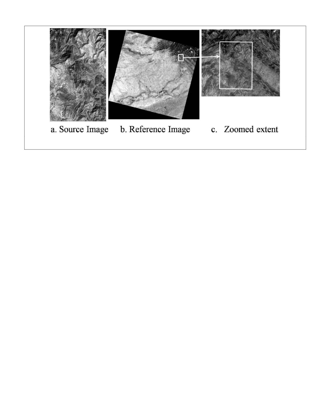
To substantiate the above discussed
GA
formulation, con-
trolled simulations are carried out using one of the CARTO-
SAT-2A scenes. The specifications of the source and reference
data sets used are described in Figure 4. Initially, the entire
candidate points
P = {p
i
| i
Є
1...n}
are validated manually by
inspecting both the source and reference images. The can-
didate points set
P
is split into two mutually exclusive sets
Q
and
R
, where
Q = {q
j
| j
Є
1...m}, m<n
and
R = P- Q
. The
m
points from
P
are randomly chosen and Gaussian errors
within ±15 pixels are added to all the points in
Q
and then
Figure 4. Cartosat-2A data set used for the case study and corresponding reference ortho-product of LDCM/OLI depicting the area cov-
ered (Region: Part of Northern India).
PHOTOGRAMMETRIC ENGINEERING & REMOTE SENSING
May 2016
381


