is typically mounted on a gyro-stabilized platform designed
to dampen the effects of atmospheric turbulence (Lee and
Bethel, 2001; Sandau, 2010), rapid orientation changes cannot
be completely eliminated due to the imperfect performance
of the gyro-stabilized mount (Lee
et al
., 2000; Gehrke and
Uebbing, 2011). If strong turbulence is encountered, light rays
may jerk backward and forward to some extent (Gehrke and
Uebbing, 2011; Wohlfeil, 2012), and the previous iterative
search algorithms may fail to converge.
This paper presents a more robust scan-line search method
for the object-to-image projection of airborne pushbroom im-
ages. The algorithm employs a coarse-to-fine search strategy
and comprises four consecutive steps: affine transformation,
iterative search, sequential search, and sub-pixel interpola-
tion. All the parameters used in the iterative search step, such
as the iterative step size and convergence conditions, were
carefully designed to ensure the efficiency and robustness.
Mathematical Basis
Coordinate Systems
Three coordinate systems are involved in the transformation
between an airborne pushbroom image and the object space.
1. Level-0 (L0) image coordinate system.
An L0 image is a collection of consecutive scan lines
acquired by a linear
CCD
array. As shown in Figure 1,
its coordinate origin typically locates at the upper-left
corner of the image, the
x
-axis points forward along the
flight direction, and the
y
-axis points left.
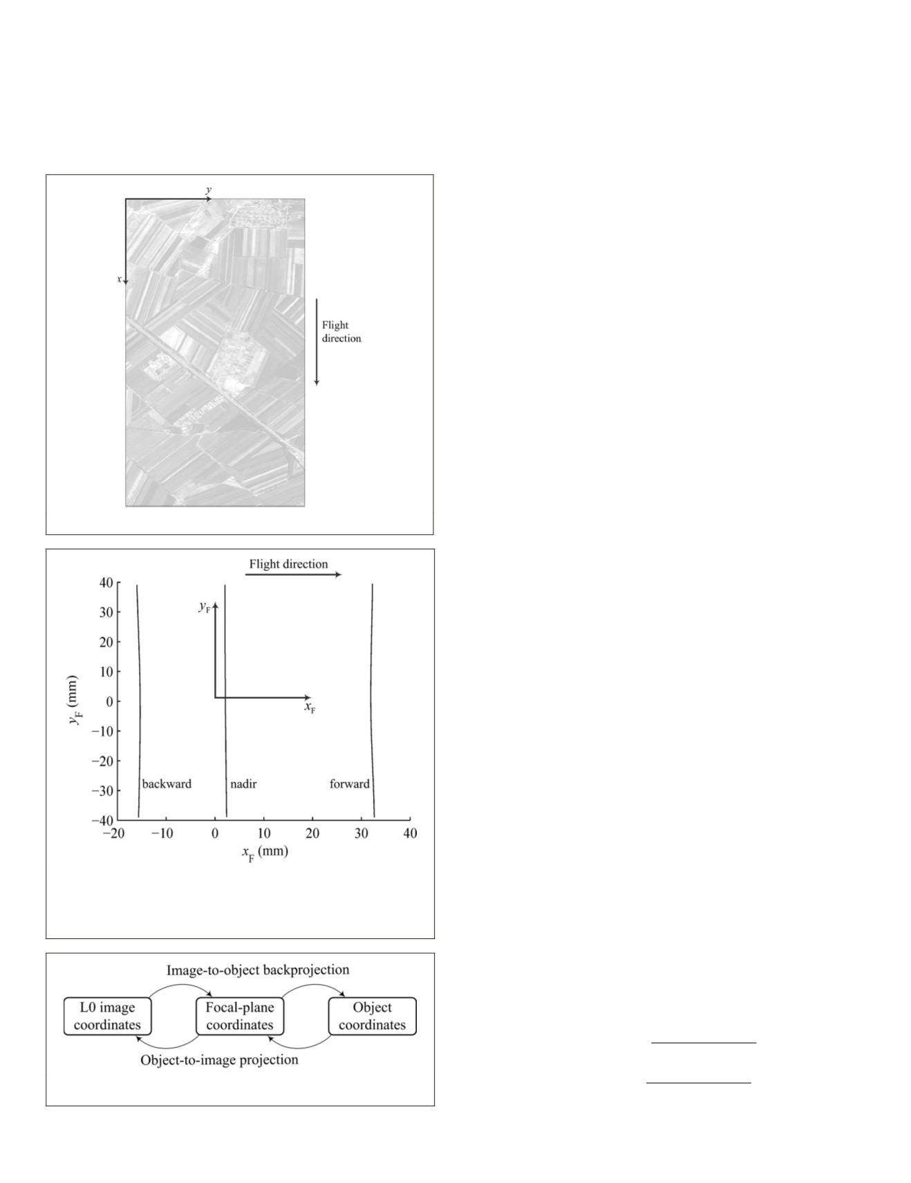
2. Focal-plane coordinate system.
The locations of linear
CCD
detectors in the focal plane
are described by this coordinate system. As shown
in Figure 2, its coordinate origin is the intersection
between the optical axis and the focal plane, and the
x
-axis and
y
-axis point forward, along and to the left of
the flight direction, respectively.
3. Object coordinate system.
This is a local space rectangular frame. Its coordinate
origin is typically set at the centroid of the block,
which is anchored to the
WG
S84 ellipsoid with an ellip-
soidal height of zero, and the axis directions follow the
east-north-up convention.
Figure 3 depicts the transformation relationships between
the L0 image coordinate system, the focal-plane coordinate
system, and the object coordinate system.
Image-to-Object Backprojection
In the processing of the image-to-object backprojection, the L0 im-
age coordinates are first transformed to focal-plane coordinates.
x
y
y
y y
y
y
y
x n
x n
x n d
y n
y n
F
F
cal
cal
cal
cal
cal
=
+
−
(
)
=
+
−
+
+
[ ]
[
]
[ ]
[ ]
[
]
1
1
cal
y n d
y y
[ ]
(
)
(1)
where (
x
F
,
y
F
) is the focal-plane coordinate to be solved;
y
n
and
y
d
are the integer and fractional parts of the
y
-coordinate
in the L0 image, respectively; the subscript (
n
+1) refers to the
next pixel of the current integer-pixel position
n
; and cal[ ] is
the two-column (
x
and
y
) look-up table formed by the focal-
plane coordinates of the
CCD
detectors.
The next step is to transform the focal-plane coordinates to
object space coordinates. As an image is a 2
D
projection of the
3
D
object space, some additional data (e.g., range observations
or terrain elevations) are required in the process. Supposing
the ground height
Z
is known, then the transformation can be
implemented by the inverse form of the collinearity equations.
X X Z Z
r x r y r f
r x r y r f
Y Y Z Z
r x
S
S
S
S
= + −
(
)
+ −
+ −
= + −
(
)
11
21
31
13
23
33
12
F
F
F
F
F
F
F
F
+ −
+ −
r y r f
r x r y r f
22
32
13
23
33
(2)
Figure 1. Level-0 image coordinate system.
Figure 2. Focal-plane coordinate system. Three panchromatic lin-
ear
ccd
arrays from a Leica ADS80 scanner are shown. It can be
seen that the locations of the
ccd
arrays are not exactly straight
on the focal plane, but are in fact slightly curved.
Figure 3. Transformation relationships between the L0 image co-
ordinates, the focal-plane coordinates, and the object coordinates.
566
July 2015
PHOTOGRAMMETRIC ENGINEERING & REMOTE SENSING


