a break in the increases of the granulometry curve. The cumu-
lative average of the
PS
is defined as:
m n
n
n
c
S j
S j
j
n
( )
,
, ,...
,
,
=
−
−
=
−
=
∑
1
1
2 3
1
2
Γ Γ
(8)
or
m n
n
n
c
S n S
( )
,
, ,...
,
,
=
−
−
=
Γ Γ
1
1
2 3
(9)
Equation 9 implies that
m
c
(n)
is the slope of the line con-
necting the origin of the granulometry curve to the point cor-
responding to
n
.
Γ
S,n
–
Γ
S,n
–1
can also be taken as the local slope
of the curve at
n
. When the local slope of the curve at point
n
is obviously higher than
m
c
(n)
,
n
is detected as
s
0
. That is,
Γ
S,s
0
–
Γ
S,s
0
–1
>
m
.
(10)
where
e
is a given value that can be close to
m
c
(n)
. The
peak scale of
m
c
can be taken as the end of the scale range,
sp
.
Here in Figure 2 the peak indicates the radius of 28, which
implies that the maximal size of the bottom of the building
dome is close to 50-by-50 pixels.
It should be noted that there may be more than one peak in
the
PS
curve. This implies that there are some other objects of
bigger sizes, such as hills or vegetation groves, existing in the
scene. The proposed technique may be not able to detect the
extremely small houses of area ranging from 5 to 10 m
2
if any.
Due to the smoothing algorithm for
s
0
detection, even there is
enough many houses of this scale, the minimal scale detected
is generally beyond 4, which equals to about 50 pixels or 12.5
m
2
in the
DSM
.
Dome Reshaping
We must label a marker for a house so that we can isolate and
extract it. After that, the gradient of the
DSM
can be watershed
segmented to determine the contours of the targets. The mark-
ers of the buildings are not expected to be very good or to be
the exact shapes of the real houses. Instead, they may appear
as “blobs.” Some houses have a general dome-like shape,
while others are more complex. As previously described ,
regional maxima can be used to extract the markers of the
buildings in case that a single height parameter is not robust
sufficiently. Alternatively, houses can be reshaped into domes
to extract the marker easily.
As we know, morphological operations change the height
and shape of an object. Therefore, we filter the
DSM
image
to change the building shapes and reconstruct the build-
ing domes to detect the markers. To this end, we propose an
iterative differential opening-based morphological filtering
algorithm, as described in Equation 11.
D
S
i
=
γ
S
i
–1
(
∏
γ
S
i
–1
(
I
) –
∏
γ
S
i
(
I
)),
i
= 1,
p
,
(11)
where
∏
γ
S
i
–1
=
γ
S
i
γ
S
i
–1
…
γ
S
0
(
I
) means the continuous
opening
of the
DSM
I
,
p
the scale range.
∏
γ
S
i
(
I
) is the dome free
DSM
at
scale
S
i
.
D
S
i
refers to disk-shaped slices of the objects at this
scale. The continuous
opening
to the
DSM
shrinks the shape of
an off-terrain object and makes it more round. Then, we part-
ly filter the object slice at a certain scale by subtracting the
opened
DSM
from the last iterative result. A house may have
several slices continuously extracted from a lower scale to a
higher scale. The scales of the slices of different houses can
vary. The sizes of the
SE
used in this stage are identical to the
scales detected in the Building Scale Detection Section. Some
thin edges will remain after differencing, which correspond
to the outside of the non-rounded objects. An opening is used
again to erase this noise from the filtered objects. This reshap-
ing operation can separate the connected houses in
DSM
, if
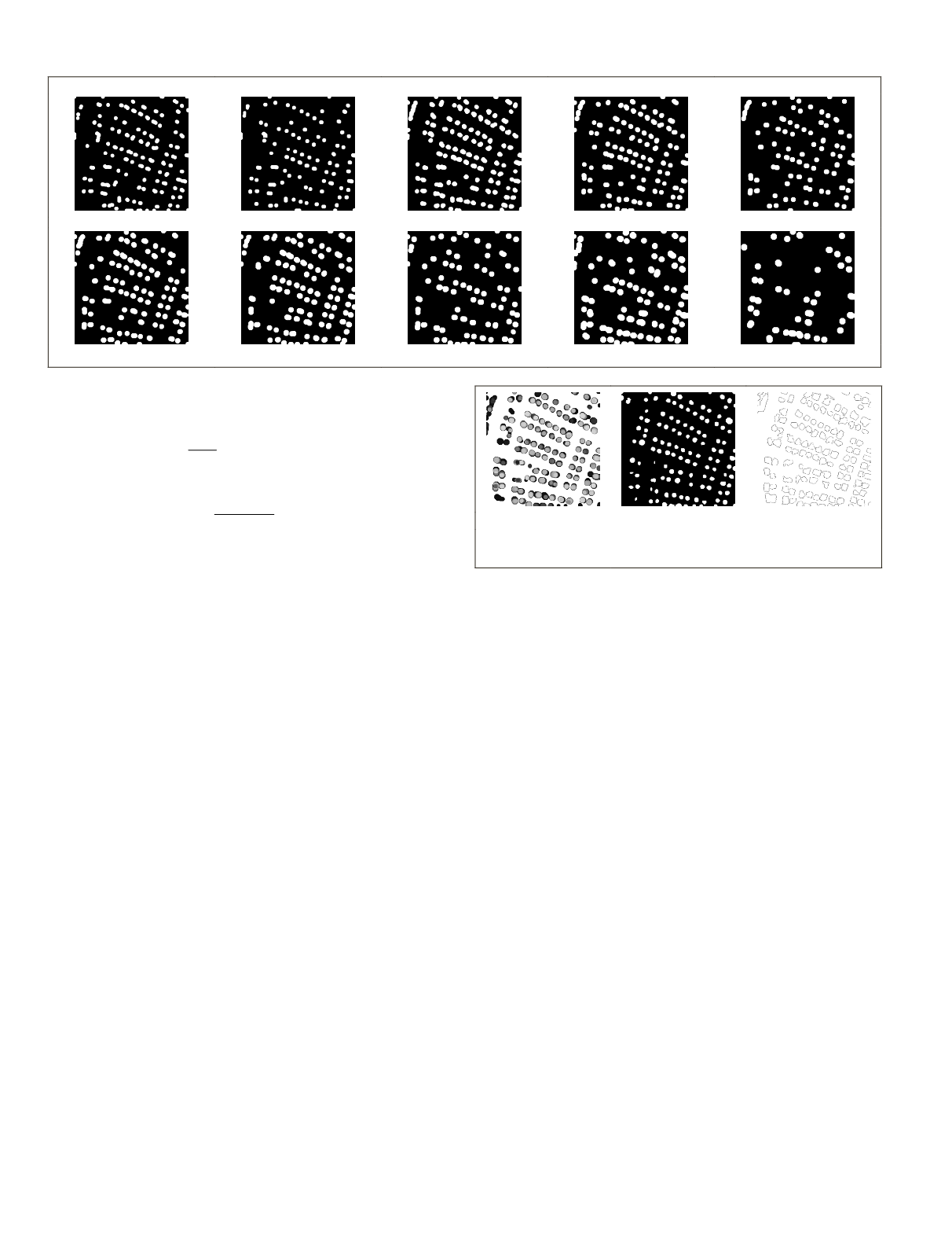
only the heights of the roofs differ. The filtered slices for the
example of Figure 2a at varying scales are shown in Figure
3. Each map in Figure 3 corresponds to the extracted slices
of the buildings at the certain scale
S
i
. The object domes are
reconstructed from these slices using
D D
S
i
S
i
=
=
−
∑
1
1
(12)
where
D
is a new gray level image that contains the reconstruct-
ed object domes, as shown in Figure 4a. Then the building
markers, as shown in Figure 4b, are extracted using the union
of local maxima (
R(D)
) and regional maxima (
ER(D)
) ; that is:
M
=
R
(
D
)
È
ER
(
D,h
).
(13)
se = 17
se = 18
se = 20
se = 21
se = 22
se = 23
se = 24
se = 25
se = 27
se = 28
Figure 3. Extracted slices at various scales.
(a)
(b)
(c)
Figure 4. The morphological computation results:
(a) reconstructed houses, (b) markers, and (c) masks.
24
January 2016
PHOTOGRAMMETRIC ENGINEERING & REMOTE SENSING


