Mask Extraction
The markers present as a round spot that indicates the basic
location of a building. A mask is defined as a region that cov-
ers the basic extent of a building. We used watershed seg-
mentation on the gradient of the
DSM
(
GDSM
) to generate the
building masks, by setting the markers as the local minima of
the
GDSM
(i.e., the catchment basins). The classic immersion
algorithm proposed by Vincent and Soille (1991) can give the
desired result. The mask map for the test data in Figure 2a is
shown in Figure 4c.
Most of the generated masks correspond to houses, while
some may correspond to trees and others. They can be rec-
ognized using an image transform. Many authors had shown
objection about the effectiveness of using
NDVI
(Awrangjeb
et
al
., 2012). We also found that in very high resolution imagery,
NDVI
as shown effective for vegetation detection in medium
resolution cases cannot recognize vegetations very well. In our
case, the near infrared image is not available thus other index
for vegetation should be developed. Some people suggest that
use green index (green channel) instead of the infrared channel
to detect the vegetation. But when using (
R
-
G
)/(
R
+
G
), shadows,
shady side of roofs and some light blue roofs will also be de-
tected together with trees. In regard to this, we propose to use a
texture index and a spectra based normalized greenness index
to classify vegetation and others. The texture index of an object
is defined as the standard deviation of the
DSM
of the object.
Trees generally have bigger texture values than general roofs.
The normalized greenness index is defined as
G
/(
R+B
), which
is effective to strengthen the green component among the red,
green, and blue components. Trees generally have bigger green-
ness values than general roof. A high texture pixel is detected
if its texture value is greater than the binary threshold, which
is derived by Otsu’s algorithm. Similar with a high greenness
pixel. A tree object is detected if the sum of its high-texture-
pixel-ratio and its high-greenness-pixel-ratio greater than 1.
Results and Evaluation
The effectiveness of the proposed method was investigated
using some experimental results on Japanese test datasets. We
clipped several image patches and the corresponding DSMs
of Tokyo and Sapporo to construct three datasets, which con-
tained various types of house distributions.
Extraction Results
The
DSM
of Dataset 1 is shown in Figure 2a, which is the data
that we used to interpret our method in previous parts of this
paper. Their markers and masks in Figure 4b and 4c, respec-
tively, show that most of the houses were correctly labeled
and separated. The pure spectral objects that were segmented
from the multiple-spectral image and overlapped by a mask
have been grouped and merged into the footprint of the cor-
responding building, and modeled as a regular polygon. The
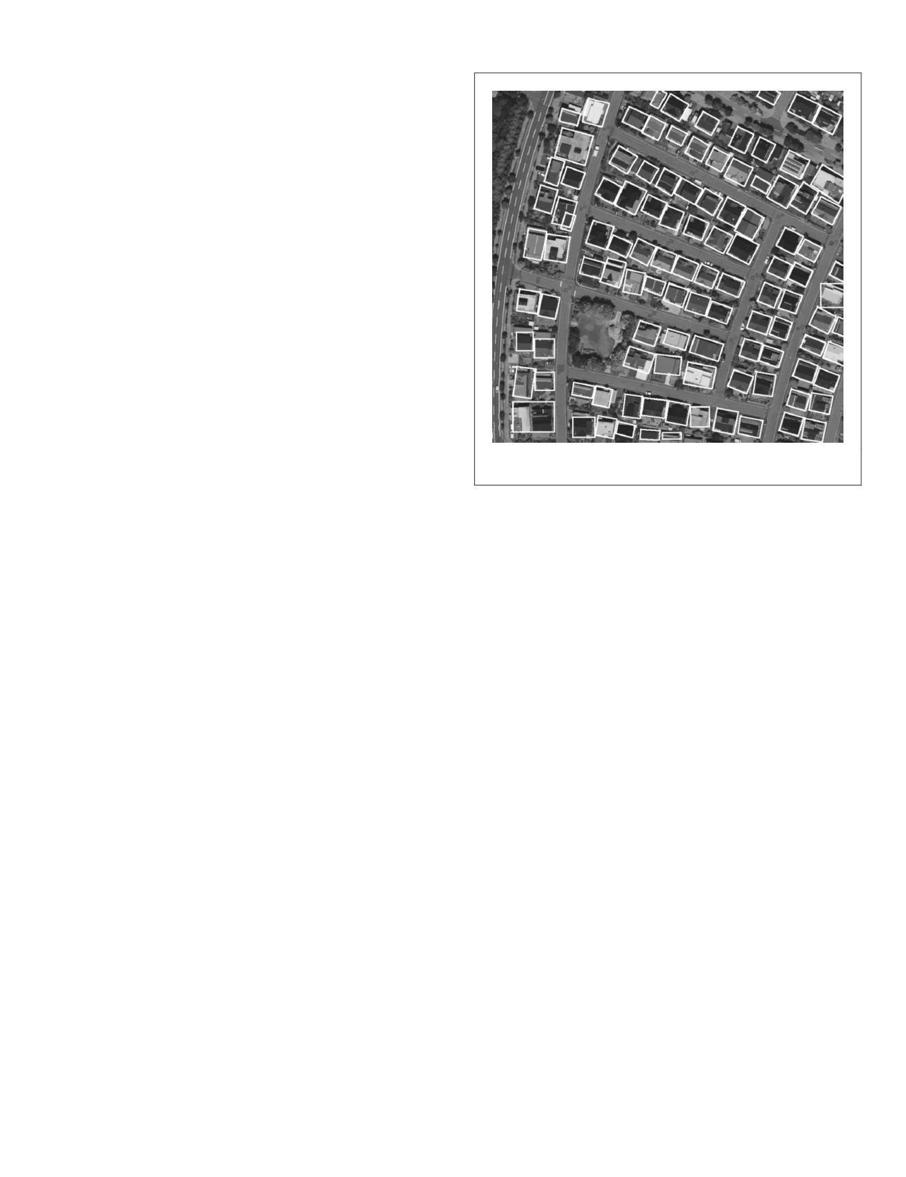
rectangular models of the houses are shown in Figure 5. They
were generated by orientation estimation and polygon refin-
ing using the edges of the footprints, as introduced in Li
et al
.
(2012). It can be seen that the models fit the houses very well,
in terms of both the orientation and the size.
The
DSM
of Dataset 2 is shown in Figure 6a. which is
another part of Sapporo. It contains high-density residential
housing and large warehouses (which can be detected using
segment area criteria based on the image). The big build-
ings do not need markers or masks for modeling. They were
detected and extracted directly from the image segments,
and modeled in the same way as the small houses. Figure 6b
shows the rectangular restrained polygon models superim-
posed on the
RGB
image for Dataset 2. Most buildings were ex-
tracted and modeled correctly; very few houses were missed.
Two neighboring houses were mixed during the extraction
process. The
DSM
of Dataset 3 is shown in Figure 7a, which
presents a region of Tokyo. Different from the former two da-
tasets, it contains high-density but disordered houses. Figure
7b shows the rectangular restrained polygon models super-
imposed on the
RGB
image for Dataset 3. Several houses were
missed because no markers were extracted for them. Some
houses were not modeled in correct directions.
Comparison with Other Methods
To prove the house detachment ability of the proposed
method, we compared it with other methods in terms of some
simple metrics using Dataset 1. The methods include marker-
controlled watershed segmentation and Pesaresi’s segmenta-
tion method. The mask map derived from marker-controlled
watershed segmentation is shown in Figure 8b. The markers
were detected by the local maxima of the smoothed
DSM
. It
can be seen that some masks do not fit the buildings very
well. There are some errors at the bottom left because of the
small
SE
used for smoothing. But if we increase the size of the
SE
, the houses in the upper part of the
DSM
will connect to
each other. The mask map derived from Pesaresi’s segmenta-
tion is shown in Figure 8c. Pesaresi’s method segments the
image or
DSM
using the multiple-scale
DMP
. It generates a
DMP
for each pixel by both opening-by-reconstruction and closing-
by-reconstruction. The maximal value is chosen as the convex
scale or concave scale for the pixel. The convex segmenta-
tions correspond to the off-terrain objects, as shown in Figure
8c for Dataset 1. The main problem is that the scale range
used for
DMP
generation is not certain, and various ranges
will cause completely different segmentations. Here, a scale
range from 1 to 10 for the
SE
is chosen for
DMP
generation. In
our method, we do not have this problem because the scales
of the objects are detected by the granulometry. As Figure
8c shows, the objects yielded from Pesaresi’s segmentation
method were composed of spatially connected pixels with the
same scale. There were many connected objects. The diffi-
culty is to decide which connected objects represent the same
house and should be merged.
We took an object-based evaluation to compare the detail
extraction performance of the proposed method with other
Figure 5. Models of the buildings superimposed on the RGB
image of Dataset 1.
PHOTOGRAMMETRIC ENGINEERING & REMOTE SENSING
January 2016
25


