The Interior Orientation Parameters Adjustment
According to the Equation 6, the principal distance
c
can be
computed through a pair of orthogonal vanishing points. But
different principal distances are obtained by different pairs of
orthogonal vanishing points, and a set of principal distances
F
= {
c
1
,
c
2
…
c
n
} can be derived. Theoretically, the variance of
F
should be minimal when the principal point is at the accurate
position. Conversely, the variance is larger when the principal
point away from the accurate position is father. Hence, Equa-
tion 6 is the observational equation of all pairs of orthogonal
vanishing points. The unknown parameters are the principal
point
c
and the principal distance (
x
0
,
y
0
). Similarly, they can
be solved by using a least squares adjustment.
Loop Optimization
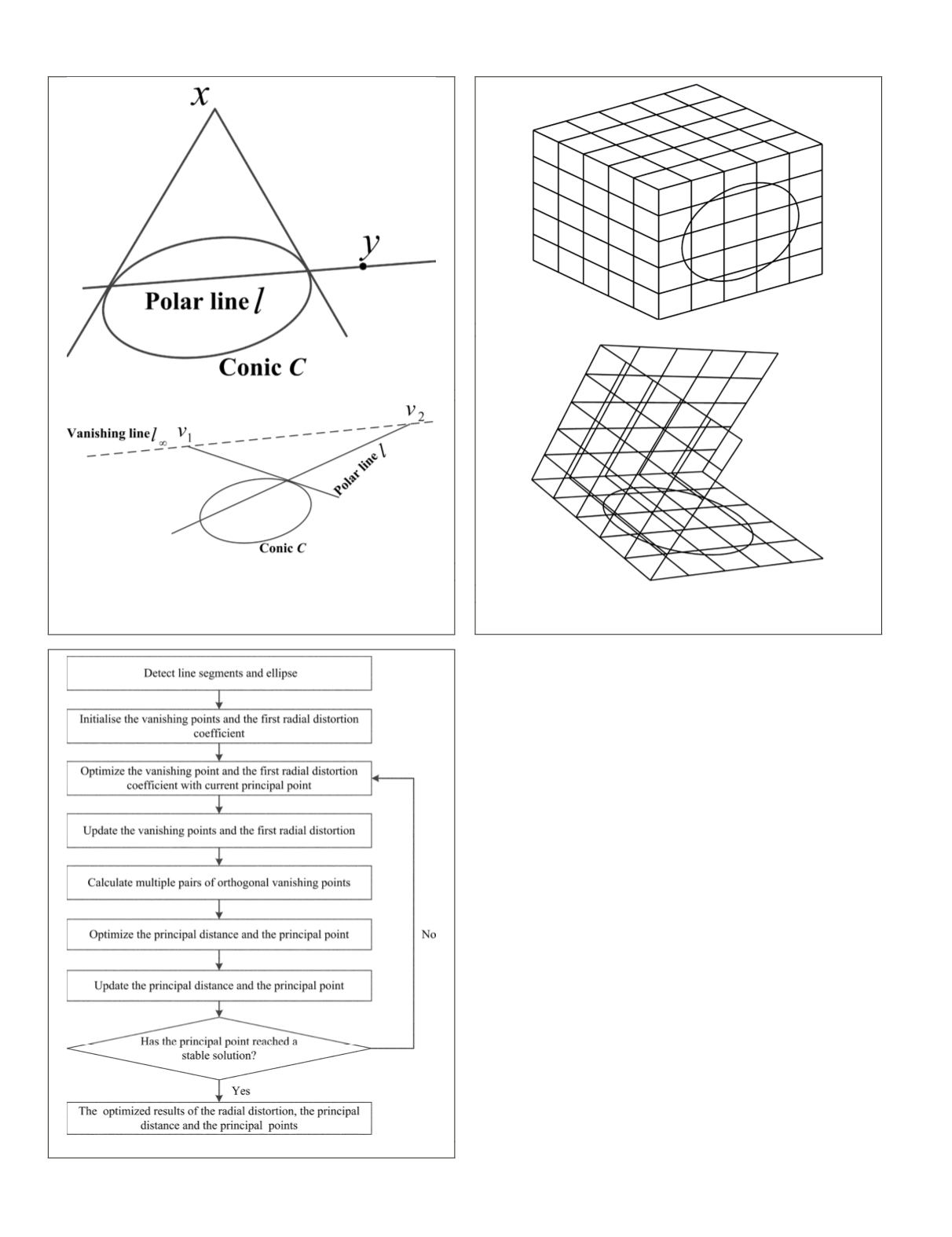
To further improve the results of self-calibration from a single
image, the distortion center is considered by repeating the two
processes of the distortion correction and the interior orienta-
tion parameters calculation. Loop iteration is used to optimize
the first radial distortion coefficient, the principal distance,
and principal point. Starting the iteration process the distor-
tion center is set as the image center. Now the first radial
distortion coefficient and interior orientation parameters can
be estimated by the Equations 5 and 6, respectively. The next
step is to improve the accuracy of the distortion center, i.e.,
the principal point; assuming the principal point calculated
so far is true, and using the current principal point as the dis-
tortion center. Then, the processes of distortion correction and
the interior orientation parameters calculation are iteratively
continued until the principal point does no longer change
significantly. The whole algorithm is illustrated in Figure 4.
(a)
(b)
Figure 3. Orthogonal vanishing point pairs computed by the
pole-polar relationships: (a) the pole-polar relationship, and (b)
Orthogonal vanishing point pairs.
Figure 4. Flow chart of the algorithm.
(a)
(b)
Figure 5. Data of simulated experiments: (a) Simulated spatial
data, and (b) Projected image data.
328
May 2016
PHOTOGRAMMETRIC ENGINEERING & REMOTE SENSING


