wherein horizontal direction
m
x
(
P
i
) and
V
x
(
P
i
) are calculated
in the similar way as Equations 4 and 5.
N
represents the
total number of pixel number of the image and
w
c
(
C
i
,
C
J
) is the
weight, calculated by Gaussian function in Equation 6:
w C C e
c
i
j
C C
i
j
c
( , )
=
−
−
2
2
2
σ
(6)
To decrease the computation complexity, all the colors of
an image are quantized to a set of M colors and get {
Q
m
}
m
=1
.
Accordingly, the spatial center and variances of quantized
color can be calculated as follows:
m P
w Q Q
y
h w Q Q
y i
c
k j
i
y
j
j
c
k j
j
M
iCi Qj
'( )
( , )
,
=
⋅
⋅
(
)
∀
=
=
→
∑
∑
∑
1
1
M
(7)
⋅
−
V P
w Q Q
y m p
h w Q Q
y i
c
k j
i
y i
y
j
M
j
c
k j
j
iCi Qj
'( )
( , )
(
'( ))
( , )
=
⋅
∀
=
→
∑
∑
2
1
=
∑
1
M
(8)
where
C
i
Q
m
indicates that the original color of pixel (x
i
, y
i
) is
quantized to the
m
th
bin of the new quantized color histogram.
Calculate Saliency Probability Map
The probability of a pixel belonging to saliency object
Prob(P
i
)
is calculated by a multivariate Gaussian function as follows:
Pr ( )
exp(
)
ob P
g
g
i
i
T
i
=
( )
−
−
(
)
−
(
)
∑
∑
−
1
2
2
2
1
π
µ
µ
(9)
g
V p
n
V p
n
m p n
n
m p n
n
i
x i
w
y i
h
x i
w
w
y i
h
h
=
⋅
⋅
−
−
12
12
2
2
'( )
'( )
'( )
'( )
T
(10)
µ
=
=
0 5555
0 6449
0 0002
0 0063
0 0231 0 0010 0 0001
.
.
.
.
.
- .
.
- .
- .
.
- .
.
.
- .
.
.
0 0002
0 0010 0 0246 0 0000 0 0000
0 0001 0 0000 0 0115 0 0003
0 0002 0 0000 0 0003 0 0080
- .
.
.
.
∑
(11)
where
N
w
and
n
h
are the width and height of the image, re-
spectively..
Results and Discussion
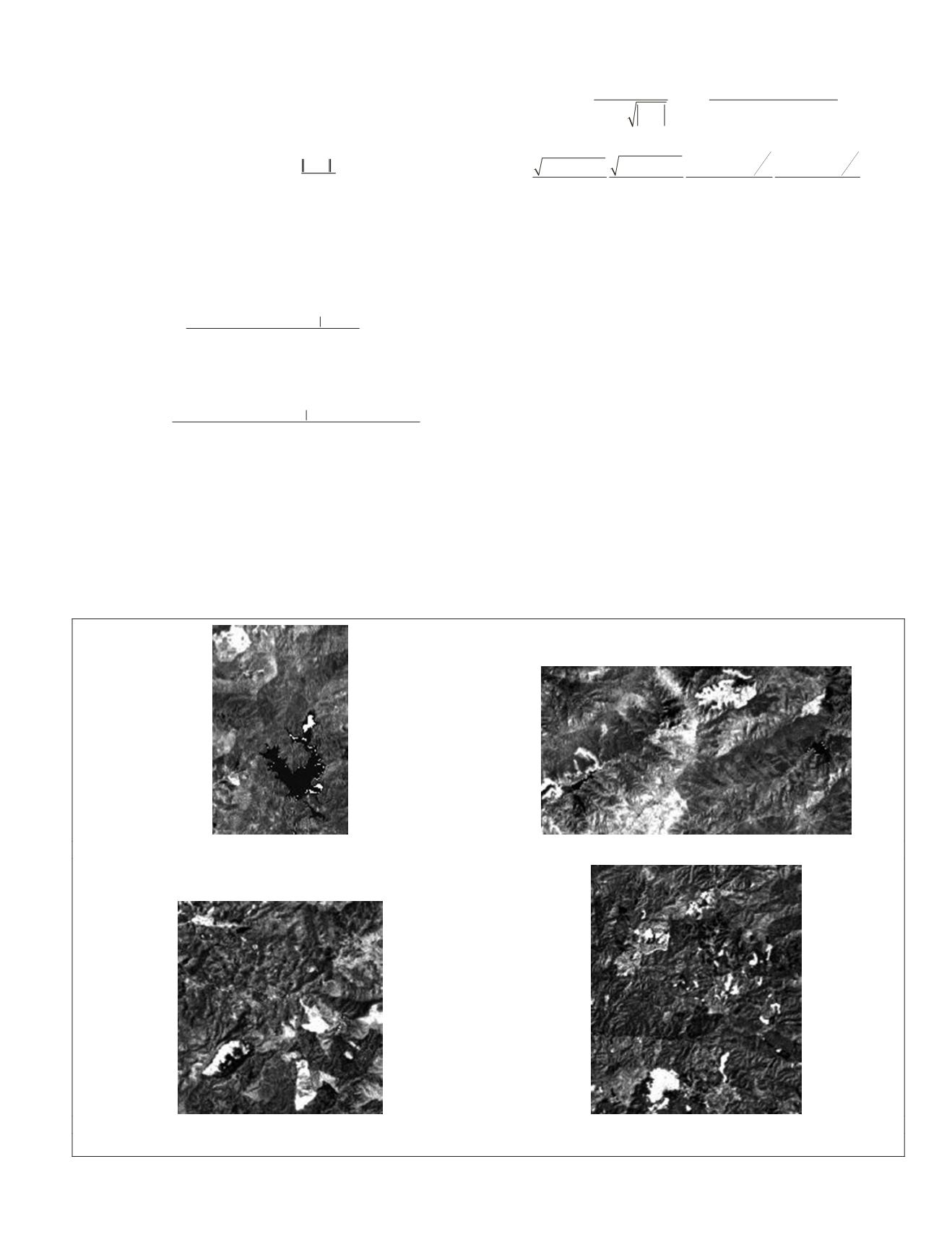
After calculating saliency probability maps, we rescaled them
to 0-255 and demonstrated in Figure 7.
Referring to pre- and post-landslide images in Figure 4,
the landslide region has been obviously highlighted as a
saliency object in Figure 7, and the background vegetation has
been largely suppressed. Calculating saliency probability of
each pixel being landslides makes landslide detection easier,
because saliency is calculated to enhance the regions whose
color, texture, and spatial characteristics are largely different
from neighboring regions. In terms of change detection using
inverse
NDVI
, the regions where landslides occur have greater
(i)
(j)
(m)
(n)
Figure 6.
Continued from last page.
PHOTOGRAMMETRIC ENGINEERING & REMOTE SENSING
May 2017
357


