PE&RS May 2017 Full - page 368

of the extracted spectral signatures and then select the most
spectrally neutral reference as a flat field.
An ideal flat field might not be available within the study
scene, and in such a case researchers need to accept the best
available flat field, that is, as in this case. For urban studies,
finding ideal flat field covering sufficient number of pixels is
a practical difficulty. Ideal flat fields such as playas, salt flats,
dam faces, sand beaches (Clark et al. , 2002) are not very com-
mon elements of an urban scene. Salt flats and sand beaches
might be a part of a coastal city scene, but that is not the case
for inland cities. Because of these difficulties, urban covers
such as open areas (in undeveloped region), play grounds,
building construction sites, concrete pavement (e.g., parking
lots), residential and industrial roof covers are a few impor-
tant candidates for flat fields within the urban scene (Desh-
pande et al., 2014). To the best of our knowledge, there are
only limited studies for flat field assessments (Clark, et al.,
2002) and few in urban settings.
Physics-Based Methods
EO-1 Hyperion Equation for Clear Atmosphere
The Unites States Geological Survey (USGS, 2011) provides a
simplified formula for converting radiance values to reflec-
tance values in relatively clear atmospheric conditions:
ρ π
θ
λ
λ
p
s
L d
ESUN
= .
. cos
2
(3)
where, ρp is reflectance, Lλ is spectral radiance at the sensor, d2
is Earth-Sun distance in astronomical units, ESUNλ is Hyper-
ion solar irradiance, and θs is solar zenith angle in degrees
(USGS, 2011).
Second Simulation of a Satellite Signal in the Solar Spectrum (6S/V)
6S is widely used radiative transfer code that provides simula-
tion of satellite signal accounting for elevated targets (Vermote
et al., 2006). One of the practical advantages of 6S is that it
provides standard atmosphere and aerosol models. These
models can be then used for atmospheric correction in ab-
sence of accurate field measurements. 6S provides comparable
or better results than similar radiative transfer codes available
(Kruse, 2004; Zhao et al., 2000; (Lee et al., 2015).
We used a python interface (Wilson, 2012) to calculate
the reflectance calibration constants namely xa, xb, and xc
(Vermote et al., 2006; Zhao et al., 2000). Corrected reflectance
is then calculated as:
y = xa × Li – xb (4)
acr y
xc y
= + × 1
(5)
Where, Li (W/m2 SR µm) is measured radiance for a given
satellite band i.
Classification
Spectral Angle Mapper
SAM is one of the simplest and important methods for classi-
fication of pixels in unsupervised manner that may use refer-
ence signatures from the field or the spectral library (Kruse et
al., 1993). The objective is to identify the target pixel material
by comparing the spectrum of that pixel with the spectrum of
known material. The pixel can be assigned a material class if
the pixel spectrum matches with a particular reference spec-
trum of the known material. The degree of matching between
target spectrum and reference spectrum is given by the angle
between the two spectral vectors of m dimensions, where m is
the number of bands in a spectrum. Formally, cosine of angle
between pixel vector and a reference member is given by:
cos( )
.
θ = l pi j
|| li||||pj|| (6)
where, θ = angel between pixel vector and reference vector,
L = {li=1, l2, l3, …, ln ,} = set of spectra of references, l1, l2, …, ln
= reference spectra; say for example, each member represent
signature for asphalt, concrete, gravel surface and so on. li =
{rk=1, r 2, r3, …, r m,} = vector of reflectance values in each band;
m = number of bands, pj = {r k=1, r2, r 3, …, r m,} = m dimensional
pixel spectral vector (Deshpande et al., 2013).
Overall Procedure
Two Hyperion images on path 147 and row 47 with scene
centers 18.5020 N, 73.8151 E and 18.5020 N, 73.7457 E were
acquired (USGS, 2013a), (USGS, 2013b). Coverage of ~25 km2 is
required for entire Pune City, Maharashtra, India which is cov-
ered by three Hyperion images (each 7.7 km wide). We focused
on the western fringes of the city as the area that has seen tre-
mendous urbanization in the recent past because of emerging
information technology hubs (Deshpande et al., 2013).
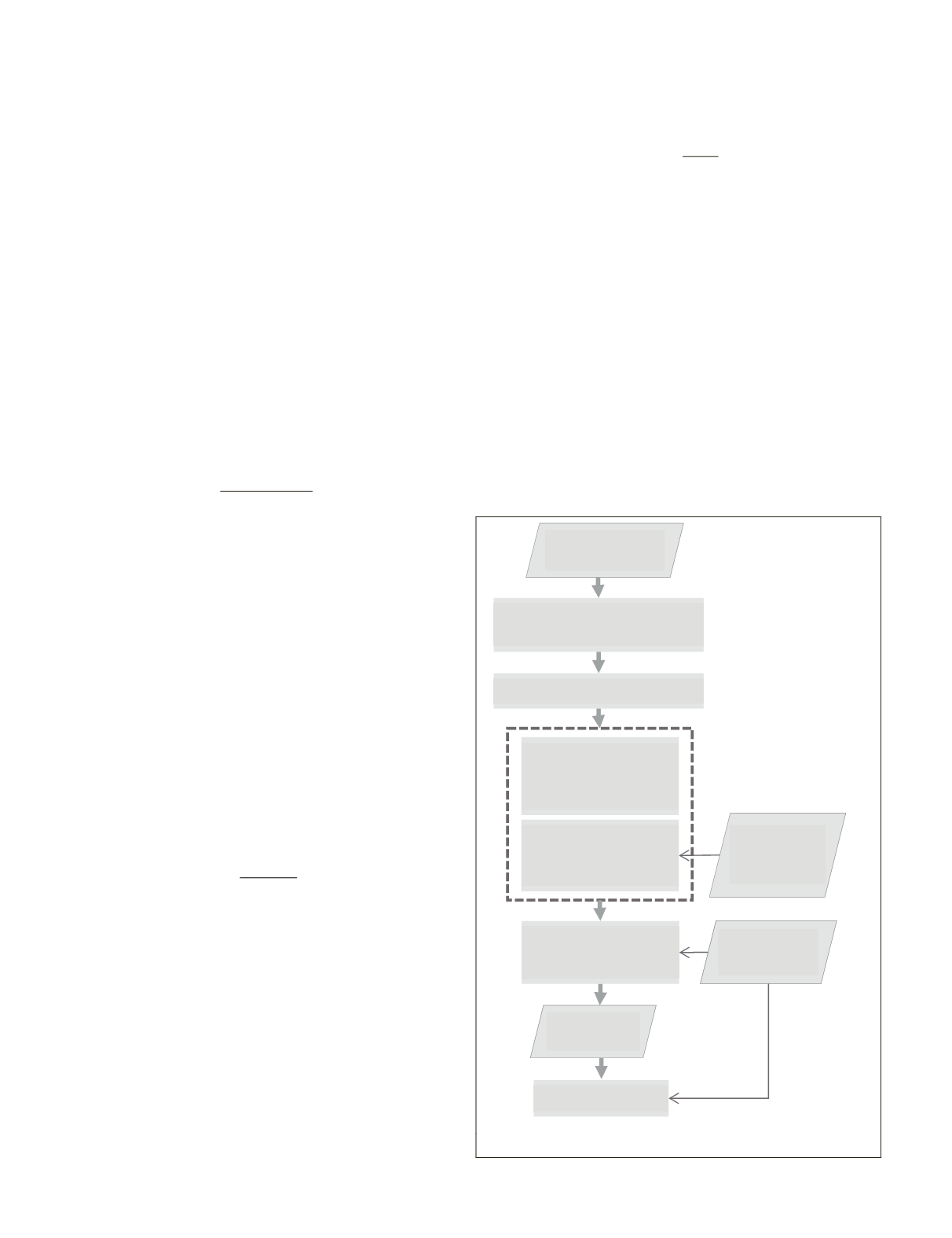
The procedure for calibration and classification begins
with conversion of Digital Numbers (DNs) to radiance values
Convert radiance to
reflectance using
6SV, EO-1 equaƟon
Training and
TesƟng data
ClassificaƟon
results
Remove uncalibrated and
water absorpƟon bands
Classify target
signature using SAM
AddiƟonal
atmospheric
data
Convert DNs to radiance
Convert radiance to
reflectance using
IAR/FAR
Evaluate results
EO1-Hyperion
image
Figure 2. Overall methodology for classification of urban LULC.
368 May 2017 PHOTOGRAMMETRIC ENGINEERING & REMOTE SENSING