surrounding air masses of high pressure flow to the center.
The upward airflow is consequently formed in the center,
which is beneficial for the diffusion of pollutants. On the
contrary, when the ground is dominated by high pressure, the
center area has downward airflow which impedes the dilution
and diffusion and thus increases the concentrations of pollut-
ants. In Hong Kong, northwest wind often occurs in winter
and brings the pollutants from
PRD
region leading to the
increase of
PM2.5
concentrations, while southeast wind from
the South China Sea brings clear air to Hong Kong. When the
temperature increases, the air convection at the lower surface
becomes stronger, which benefits the upward transport of
particulate matter and decrease its concentrations. In the
low humidity condition, the hygroscopic growth of particle
causes
PM2.5
concentrations to increase. In the high humidity
condition, the particles grow too heavy to stay in the air and
dry deposition occurs. As a result, particle numbers diminish
and
PM2.5
concentrations decrease. High wind speed acceler-
ates the diffusion of
PM2.5
, whereas low wind speed inhibits
the diffusion of
PM2.5
and makes the
PM2.5
accumulate at the
surface. Secondly, large road length indicates dense traffic,
which is one of main sources of
PM2.5
. In high
NDVI
area, the
density of traffic and population is low and the vegetation can
purify the air. Therefore, the
PM2.5
concentration is low.
Moreover, we investigated the goodness-of-fit of all models
in terms of R
2
and
AIC
(Akaike Information Criterion). The
R
2
of
GWR
-based models (0.609, 0.748, 0.801 for
GWR
,
GTWR
,
IGTWR
, respectively) are higher than that of
OLS
(0.554).
AIC
is an estimator of the relative quality of statistical models for
a given set of data (Akaike, 1974). The smaller the
AIC
is, the
better goodness-of-fit of the model will have. The
AIC
values
in Table 3~6 further demonstrate that the
GWR
-based models
have better fitting than
OLS
. Among
all the models,
IGTWR
performs best
with largest R
2
and smallest
AIC
.
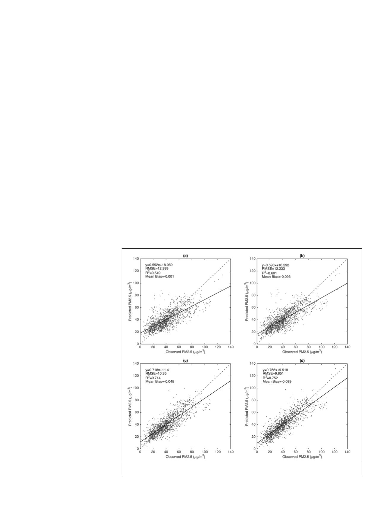
Model Validation
Cross-validation (
CV
) is a usual
way of using countable samples to
evaluate model performance (Zou
et al.,
2016). In this paper, we use
leave-one cross-validation to assess
the prediction performance of
OLS
,
GWR
,
GTWR
, and
IGTWR
. The deter-
mination of coefficients (R
2
), the
root-mean-squared error (
RMSE
), and
the mean bias between estimated
PM2.5
and observed
PM2.5
are calcu-
lated as the validation statistics.
The samples size (N = 1478)
for model validation is same with
the model fitting process. Figure 3
displays the scatter plots between
the predicted and observed
PM2.5
concentrations. The dash line is
one-one line and the solid line is
the regression line. The R
2
of
OLS
,
GWR
,
GTWR
,
IGTWR
between pre-
dicted and observed
PM2.5
are 0.549,
0.601, 0.714, 0.752, respectively,
indicating that
PM2.5
predictions
from
IGTWR
have the best agreement
with the observations. As a measure
of prediction precision, the
RMSE
of
OLS
,
GWR
,
GTWR
,
IGTWR
are 12.999,
12.233, 10.35, 9.651 μg/m
3
, respec-
tively. In summary, the local regres-
sion models (
GWR
,
GTWR
,
IGTWR
)
have better performance in
PM2.5
prediction compared with global model
OLS
.
GWR
performs
better than
OLS
by integrating spatial non-stationarity of
PM2.5
concentrations. Since
GTWR
combines both spatial and tempo-
ral effects, R
2
of
GTWR
is higher and
RMSE
is lower than
GWR
.
Among the four models,
IGTWR
has the most accurate predic-
tion with highest R
2
and lowest
RMSE
by additionally account-
ing for seasonal effects of
PM2.5
based on
GTWR
.
Annual PM2.5 Concentration Estimations
As the
IGTWR
model has been demonstrated to have better
accuracy than
OLS
,
GWR
, and
GTWR
, it is applied to predict the
averaged
PM2.5
distribution from 2012 to 2014 using corre-
sponding
AOD
, meteorological, and land use datasets. Figure 4
presents the annual mean maps of
PM2.5
concentrations based
on
AOD
available days from 01 January 2012 to 31 December
2014 and the observed
PM2.5
concentrations on ground sites
as a reference. As can be seen from Figure 4, the mean
PM2.5
concentrations of three years in Hong Kong range from 26 μg/
m
3
to 43 μg/m
3
. The annual mean
PM2.5
maps predicted by
IGTWR
for individual year reveal that the
PM2.5
level in Hong
Kong increases from 2012 to 2013 and has a decline in 2014,
which is consistent with the report of
PM2.5
trend during 1997-
2015 (Environmental Protection Department). The decline in
2014 might be a result of the Hong Kong government policy for
tackling roadside air pollution and clean air plan. From Figure
4, we can see that the distribution of estimated
PM2.5
con-
centrations from
IGTWR
is generally consistent with observed
values at sites, whereas the
PM2.5
maps from
IGTWR
provide
more comprehensive information of spatial distribution than
ground-based
PM2.5
. As expected, highly polluted areas are
found in the districts (Sham Shui Po, Kowloon City, Yau Tsim
Mong, Central and Western, Wan Chai) with sparse vegetation,
heavy population, and low altitude while districts of low
PM2.5
Figure 3. Scatterplots between
CV
prediction of
PM2.5
and observed
PM2.5
: (a)
OLS
, (b)
GWR
,
(c)
GTWR
, and (d)
IGTWR
(Dash line: one-one line, solid line: regression line).
766
December 2018
PHOTOGRAMMETRIC ENGINEERING & REMOTE SENSING


