interpolate a 1 m raster bare earth
DEM
from returns classified as
terrain points by each respective organization. A comparison of
lidar data collection methodologies is in Table 1.
Digital Terrain Analyses and GPS Data Collection
All digital terrain analyses were conducted using System for
Automated Geoscientific Analyses (
SAGA
, version 2.1.0) and
ArcGIS
©
(ArcMap, version 10.1) software.
GPS
data were col-
lected using a Trimble Geo XT 2005
GPS
unit equipped with a
Trimble Hurricane Antenna and differentially corrected using
Trimble Pathfinder software and Continuously Operating Ref-
erence Station (
CORS
) data from the National Geodetic Survey
to obtain approximately 1 m precision of horizontal positions.
DEM Aggregation, Filtering, and Sink Filling
Both the
NCALM
and
WMNF
1 m
DEMs
were aggregated to
coarser resolutions of 3, 5, and 10 m using mean cell aggrega-
tion to create eight
DEMs
. Mean cell aggregation was achieved
by computing the mean value for a designated cell neighbor-
hood, then creating a single cell of the original neighborhood
size and applying the mean neighborhood value. For example,
to create a 3 m
DEM
from a 1 m
DEM
, the neighborhood size is
nine cells (center cell plus eight adjacent cells). A 5 m
DEM
is
created using a 25 cell neighborhood, and a 10 m
DEM
is cre-
ated using a 100 cell neighborhood. Then, a second version
of each
DEM
was created by treating each
DEM
with a simple
low-pass smoothing filter using a mean filtering technique
for a total of 16
DEMs
. Mean low-pass filtering computes the
average elevation value in a 3 × 3 cell neighborhood moving
window and applies that value to the cell at the neighbor-
hood center. Unlike cell aggregation, low-pass filtration does
not change the size of the grid cells. Both cell aggregation and
low-pass filtration are common methods of
DEM
smoothing,
but a comparison of the effects of the two techniques on topo-
graphic metrics and catchment delineation applied in a soil
and hydrological context is absent in the literature.
Finally, we applied a sink-filling algorithm developed by
Wang and Liu (2006) to each
DEM
resolution/filter combina-
tion, which is common in hydrologic applications that require
the derivation of flow direction and cell accumulation grids.
Watershed Boundary Delineation and Contour Line Generation
DEM
-delineated catchment boundaries were established for
each
DEM
resolution/filter combination using a differentially
corrected
GPS
point collected at a weir defining the water-
shed outlet. The single flow direction algorithm (Jenson and
Domingue, 1988) was used for flow direction during delinea-
tion. Each watershed polygon was buffered to a distance of 20
m to mitigate edge effects during topographic metric computa-
tion. Contour lines with a 3 m contour interval were generated
using the native 1 m
DEM
for each lidar dataset. Finally, each
DEM
was clipped to the corresponding buffered watershed
boundary polygon. Watershed boundaries delineated from each
DEM
resolution/filter combination were assessed for differences
in shape and area.
DEM
-derived watershed boundaries and ar-
eas were compared with a manually delineated boundary mea-
sured by compass and chain survey when
HBEF
experimental
watersheds were first established in the 1950s. The boundary
has been maintained and marked since establishment and was
checked for consistency with the original survey by walking
it with a Trimble Geo XT 2005
GPS
unit in 2011. The field-sur-
veyed boundary was used a point of reference to compare with
the
DEM
-derived watershed boundaries. Bearings and distances
from the field WS3 survey were used to create a boundary
shapefile with the weir
GPS
point used for georeferencing.
Comparison of Field and DEM Slope Measurements
We compared 75 field slope measurements with
DEM
-derived
slope values. Percent slope was measured with a clinometer 5 m
upslope and 5 m downslope from soil characterization pits and
groundwater wells along the line of maximum slope. We col-
lected and differentially corrected
GPS
locations for each pit/well
location.
GPS
accuracy of approximately 1 m was sufficient for
locating pits and wells within one grid cell in the finest
DEM
ana-
lyzed. The steeper of the upslope/downslope clinometer mea-
surements was compared with
DEM
-derived percent slope values
computed using the maximum slope algorithm (Travis
et al.
,
1975) from filtered and unfiltered 1, 3, 5, and 10 m resolution
NCALM
and
WMNF DEMs
. A scatterplot comparing field slope with
difference between field and
DEM
slope was used to determine
DEM
resolution that best simulated field slope measurements.
Total Station Ground Surveys
Terrain features (boulders, hummocky topography, and fallen
tree boles) can be considered part of the ground surface, but
it is not well-understood whether lidar classification meth-
ods label terrain features as ground or whether interpolation
algorithms smooth these features during
DEM
generation. We
conducted elevation ground surveys at four locations in WS3
in May and June of 2012 using a Sokia SET 610 total station to
determine if the lidar-derived
DEMs
reflected terrain features.
Survey sites incorporated diverse topography, terrain features,
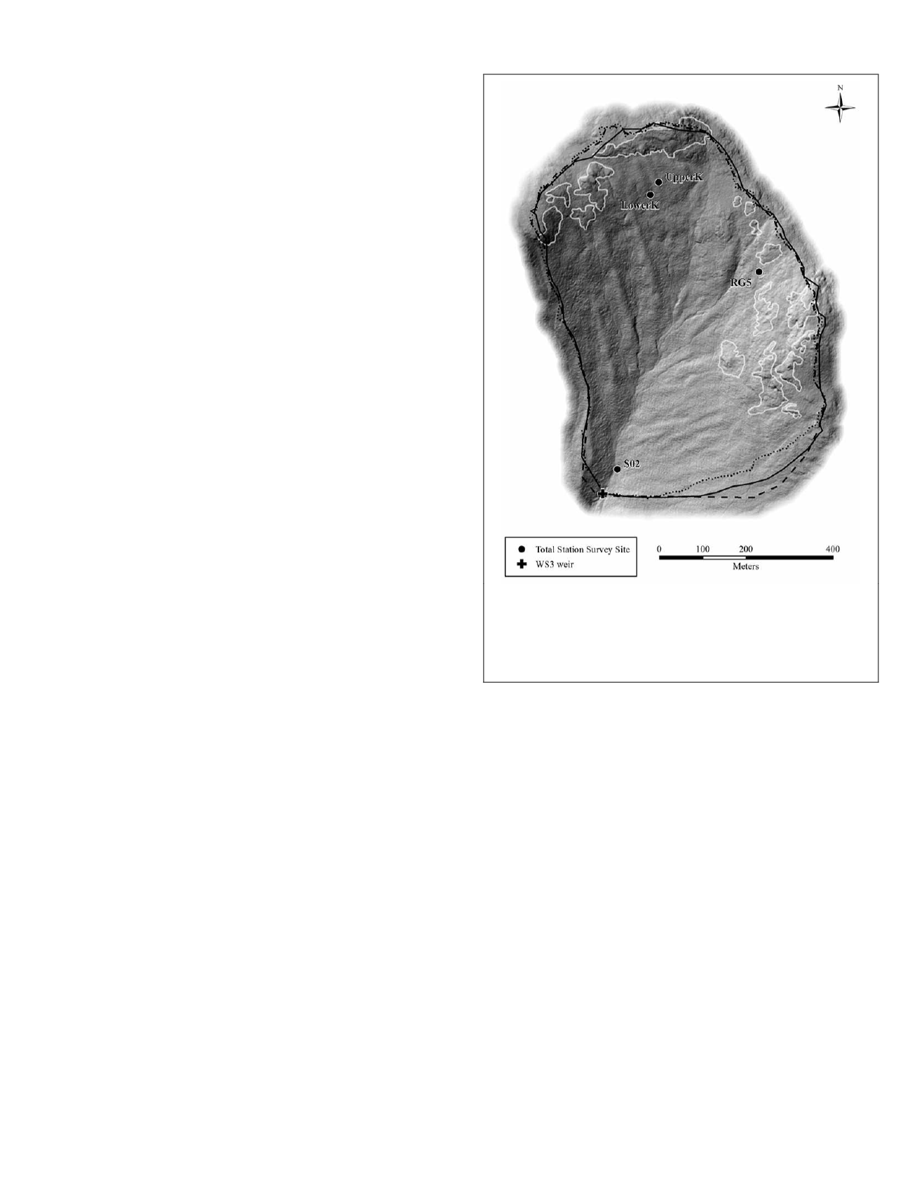
and vegetative cover. Three sites were located entirely under
mature forest canopy (UpperK, LowerK, SO2) while a fourth
site was partially located under mature forest canopy and
partially in a rain gage area cleared of mature forest but with
dense beech regrowth (RG5) (Figure 2). SO2 contained the
greatest density of understory vegetation (primarily hobble-
bush) and terrain features, RG5 contained the lowest density
Figure 2. Catchment hillshade map with total station survey sites,
catchment outlet,
dem
-delineated catchment boundaries, and
bedrock outcroppings (light grey polygons). Solid line represents
the field-surveyed catchment boundary, the small-dashed line
denotes the
ncalm
1 m boundary, and the long-dashed line repre-
sents the
wmnf
10 m boundary.
PHOTOGRAMMETRIC ENGINEERING & REMOTE SENSING
May 2015
389


