values also increased with filtering and coarsening from 4.1
to 8.4 when calculated using the
WMNF DEMs
(Figures 4c and
4d). The same overall increase in median
TWI
occurred for the
NCALM DEMs
.
TWI
distributions computed using the 3 m and 5
m
DEMs
, regardless of filtering, exhibited the greatest similarity.
Discussion
Watershed Boundary Variation with DEM Resolution and Landscape
Roughness
Each
DEM
generated a different catchment boundary. This was
especially true for the unfiltered
NCALM
1 m
DEM
, which ex-
cluded nearly 1 ha more area than the field-surveyed bound-
ary, and the unfiltered
WMNF
10 m
DEM
, which included near-
ly 1 ha more area than the field-surveyed boundary (Table 2;
Figure 2). The filtered 10 m
DEMs
from both datasets contained
nearly 1 ha less area than the field-surveyed boundary. The
area excluded or included for these four watershed boundar-
ies was chiefly located in the southeastern portion of WS3,
which is characterized by little to no channel formation and
no steep spurs compared to the rest of the catchment. Varia-
tion in catchment boundary and flow accumulation across
DEM
resolutions is consistent with previous observations (e.g.,
Quinn
et al.
, 1995; Vaze
et al
., 2010).
Such results demonstrate that care should be taken when
using lidar-derived
DEMs
for watershed delineation, especially
in regions where delineation of catchments is challenging
due to subtle topography. Uncertainty in catchment area
determination is a critical factor in evaluating catchment
water and nutrient balances as the estimate of atmospheric
precipitation inputs is dependent on this parameter. Yanai
et
al.
(2014) evaluated sources of uncertainty in stream water
flux in long-term catchment studies and noted that watershed
area has not been critically assessed at well-known long-term
catchment installations.
DEM
aggregation methods may not
adequately preserve drainage features, which affect the delin-
eation process. An important consideration from a hydrologi-
cal perspective during
DEM
generation is maintaining relative
elevation differences or drainage features (Ai and Li, 2010;
Chen
et al.
, 2012).
Agreement between DEM and Field Slope Values
DEM
-computed slope values were similar to field-measured
slope values, particularly for the 5 m and 10 m
DEMs
(Figure
3c and 3d). In this study, field slopes were measured at a 5
m scale, which helps explain why 1 m
DEMs
generated slope
values least similar to field measurements. Such results dem-
onstrate that
DEM
resolution should reflect the desired scale of
information intended for the application, e.g., operations and
management decisions, erosion modeling, or soil mapping.
The tendency for slope values to become more intermedi-
ate (decreased maximum values and increased minimum
values) with
DEM
coarsening is consistent with previous
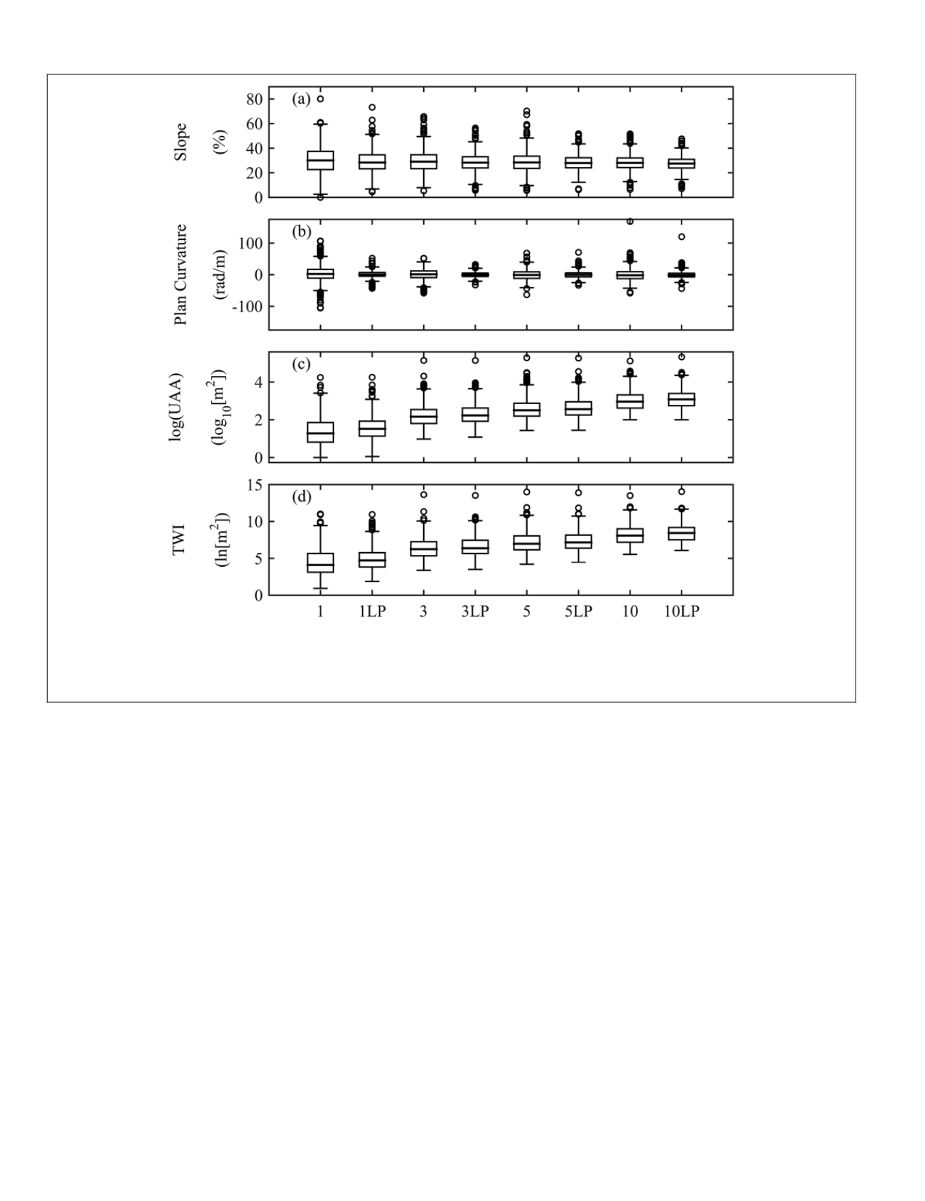
Figure 4. Box and whisker plots indicate variation in distribution of topographic metrics for
wmnf
: (a) slope, (b) planform curvature, (c)
uaa
, and (d), and
twi
. Median values are represented by the thick black line, boxes represent the interquartile range, whiskers extend 1.5
times the interquartile range beyond the interquartile range box and contain approximately 99.3 percent of the data, and circles indicate
points outside 99.3 percent of the data. Topographic metrics were computed for each
dem
and values were extracted to 421 random
points generated inside the WS3 boundary.
392
May 2015
PHOTOGRAMMETRIC ENGINEERING & REMOTE SENSING


