where,
ω
start
represents the initial
inertia weight.
ω
end
indicates the
value of the inertia weight when
the maximum number of iterations
is reached.
t
max
is the maximum
number of iterations.
t
means the
current number of iterations.
The inertia weight at the maxi-
mum number of iterations cannot
be well determined. Meanwhile, in
order to further improve the search
ability of the
PSO
algorithm, this
paper calculated the square of (
t
max
–
t
)/
t
max
and eliminated the inertia
weight at the maximum number
of iterations in the
LDIW
strategy to
improve the convergence accuracy
of the algorithm. The modified
LDIW
strategy algorithm can be
called Modified
PSO
(
MPSO
), which
is listed in the following form:
ω
=
ω
start
·(
t
max
–
t
)
2
/
t
2
max
,
(5)
In this paper, the mean square error is used as a fitness
objective function, which can be expressed as:
E X
N
Y X t
i
i
N
( )
( ( )
)
=
−
=
∑
1
2
1
,
(6)
where,
t
i
is the preoutput. The fitness function can be ob-
tained as follows:
fitness
=
+
1
1
E( )
X
.
(7)
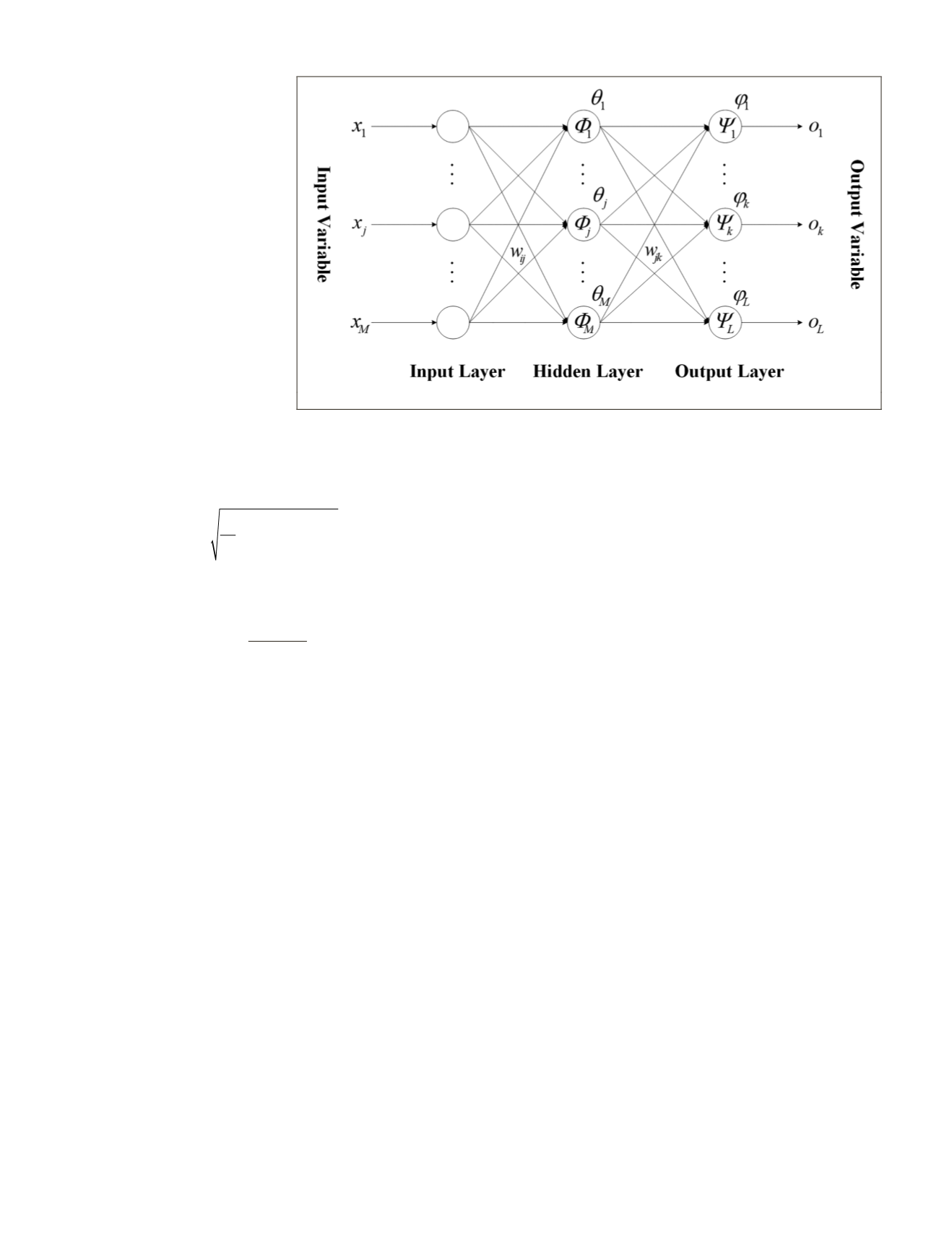
BP Neural Network
The neural network is an information processing system
based on the organizational structure and activity mechanism
of human brain. It can perform logical o
linear relationship simulation. Back-Pro
network is one of the most widely used
it is a multilayer feedforward network with error back propa-
gation algorithm (Hecht-Nielsen 1992). Figure 2 shows the
basic structure of the
BP
neural network.
In Figure 2,
x
j
represents the input parameter of the input
node,
j
= 1,2,…,
M
.
Ψ
(
x
) is the excitation function of the output
layer.
Φ
(
x
) indicates the excitation function of the hidden
layer.
w
ij
is the connection weight between hidden node and
input node,
i
= 1,2,…,
Q
.
φ
k
is the threshold of the output node,
k
= 1,2,…,
L
.
w
ki
represents the connection weight between out-
put node and hidden node.
θ
i
is the threshold of the hidden
node.
o
k
means the output parameter of the output node.
Thus, it can be seen from Figure 2 that when the
BP
neural
network is propagating forward, the input vector
net
i
of the
hidden node can be described as follows:
net
w x
i
ij j
i
j
M
=
+
=
∑
θ
1
,
(8)
Thus, the output
y
i
of the hidden node can be expressed as
follows:
y
net
w x
i
i
ij j
i
j
M
=
(
)
=
+
=
∑
θ
1
Ф Ф
,
(9)
According to the output of each hidden node, the input
vector
net
k
of hidden node is calculated as follows:
net
w y
w w x
k
ki j
k
i
Q
ki
ij j
i
j
M
k
i
Q
=
+ =
+
+
=
=
=
∑
∑ ∑
φ
θ φ
1
1
1
Φ
, (10)
The output
o
k
of the output node can be expressed as follows:
φ
θ
o
net
w y
w w x
k
k
ki j
k
i
Q
ki
ij j
i
j
M
=
(
)
=
+
=
+
=
=
∑
∑
1
1
+
=
∑
φ
k
i
Q
1
Ψ Ψ
Ψ Ф
,(11)
Moisture Retrieval
ified
PSO
and
BP
neural network algo-
ombining method (
MPSO
-
BP
) to opti-
retrieval and effectively improve the
retrieval accuracy. The optimization steps are listed as follows
(the flowchart is shown in Figure 3):
Step 1: Initializing the structure of
BP
neural network. The
number of the input and output nodes are predetermined.
The datasets used in neural network are normalized. Some
parameters including the number of training and testing
samples, the maximum number of trainings, the target error
and the number of neurons in the hidden layer are preset.
Step 2: Initializing the structure of
PSO
. The sizes of popu-
lation and particle, the initial inertia weight, the learning fac-
tors, the upper and lower limits of the position are predeter-
mined. The maximum and minimum velocity of the particle
are defined to randomly initialize the velocity of the particle.
Step 3: The fitness value of the particle is calculated and
the position of the
i
th
particle is determined as the current
optimal position
pbest
of the particle. Then, all of the fitness
values are compared to obtain the optimal position of the
population as the global optimal position
gbest
.
Step 4: According to the Equations 2, 3, and 5, the veloc-
ity and position of the
i
th
particle are updated and checked
whether they are out of bounds. Then, the fitness
f
(
x
i
) of the
i
th
particle is calculated.
f
is the fitness function.
Figure 2. Basic structure of
BP
neural network.
792
November 2019
PHOTOGRAMMETRIC ENGINEERING & REMOTE SENSING


