this specific practical scene; change within one land-cover
class is considered to be “noisy change” in our experiment.
Plate 1 shows single feature thresholding results after
T-point algorithm and their fusion results for a small subset
of the study area. The luminance image (Plate 1c) can detect
most of the conversion between built-up area and other land-
cover types. However, it over-detects some unchanged built-
up area such as the region of ‘A’ in Plate 1c. Similarly, for
saturation thresholding results (Plate 1d), there are some false
detections such as the ‘B’ region, which are actually inter-
class vegetation changes. In addition, the saturation thresh-
olding result alone is likely to miss some important changes
between built-up area and vegetation (such as ‘C’ region in
Plate 1d). Plate 1e shows that the use of the strategy of Naïve
Bayes for fusion can redetect some missed changes (such as
‘C’ region) and exclude false changes (such as ‘A’ region and
‘B’ region). For the last step, MRFs procedure allows detected
objects to be more compact, and increases reliability of detec-
tion (Plate 1f).
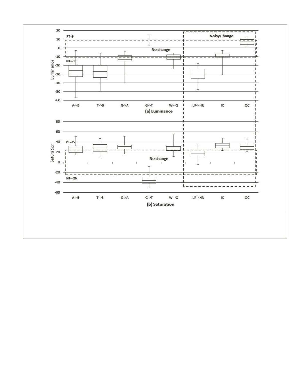
Figure 3 is a box plot based on manual samples from dif-
ferent change of interest and noisy changes, to quantitatively
confirm that luminance and saturation are complementary.
There are five land cover types in our area of change:
Built-
up Area
(
B
),
Trees
(
T
),
Grass land
(
G
),
Barren land
(
A
), and
Water
(
W
). Our change of interest is the transition between
any two of these five classes, such as from
Tree
to
Built-up
Area
(
T->B
). We selected five representative change types of
interest in our study region for making box plot:
A->B
,
T->B
,
G->A
,
G->T
,
W->G
. For noisy change in our study area, we
think they are mainly caused by local different reflectance
(
low reflectance
to
high reflectance
,
LR->HR
), quality change
of water (
QC
), or inter-class changes of vegetation (
IC
).
For every type of change, a certain number of sampling
pixels are collected according to visual interpretation. The
statistics of sampling change classes on each feature band are
shown together in the box plot; the positive (
PT
) and nega-
tive threshold (
NT
) obtained by T-point algorithm are given
to show their relationship with those change classes. The
boxplot indicates that luminance thresholding is good at
identifying the noisy change
IC
and
QC
because more than 75
percent of them fall within the “No-change” region; satura-
tion thresholding performs well in
LR->HR
; all the change
types have at least 50 percent accurate detection rates for both
two features. This result exhibits the potential of separating
change of interest from all the changes by fusing the changed
parts of luminance and saturation.
Figure 3. Box plots of feature [(a) luminance, and (b) saturation] statistics from sampled pixels, which consisted (1) 62 pixels from
Barren
land
to
Built-up area
(A->B); (2) 33 pixels of
Trees
to
Built-up area
(T->B); (3) 57 pixels of
Grass land
to
Barren land
(G->A); (4) 55 pixels
of
Grass land
to
Trees
(G->T); (5) 64 pixels of
Water
to
Grass land
(W->G); (6) 35 pixels of
low reflectance
to
high reflectance
(LR->HR);
(7) 32 pixels of inter-class change of vegetation (IC); (8) 32 pixels of water quality change (QC). Positive Threshold (PT) and Negative
Threshold (NT) were obtained by the T-point algorithm.
PHOTOGRAMMETRIC ENGINEERING & REMOTE SENSING
August 2015
641


