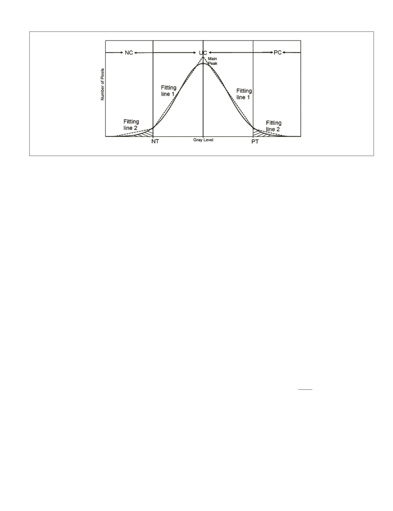
in many practical scenes. Differencing values can be negative
or positive, producing two tails in the histogram (Figure 2).
We divide the histogram curve of difference image into left
and right side by highest peak of histogram. For each side, the
T-point algorithm (Coudray
et al.
, 2010) was used to deter-
mine the change threshold. The T-point algorithm, developed
specifically for unimodal histogram through finding the best
fitting lines for each part, has been proved to be more effective
for urban areas based on our previous tests (Chen
et al.
, 2015).
It is easy to find two decision boundary, i.e., one negative
threshold (
NT
) and one positive threshold (
PT
), separating the
feature space into three classes: negative change (
NC
), positive
change (
PC
) and unchanged class (
UC
).
Bayes Fusion
Data fusion is applied in order to fuse the two class maps cor-
responding to luminance and saturation features after apply-
ing the two-sided T-point algorithm. Generally, there are two
common types for fusing two independent data band: the first
type is based on the crisp output produced by each dataset,
such as majority voting or “and/or” operation; the second
type produces the fuzzy output for each band first, and then
combine them following some rules, which is often viewed as
a better way to handle uncertainty and imprecision (Grant
et
al.
, 2008). The Bayes fusion in our proposed method belongs
to the second type.
For Bayes fusion, there are nine possible cases
l
k
for the joint
labels (
L
) based on three change results (negative change
ω
nc
,
positive change
ω
pc
and no change
ω
uc
) for each feature. Let a
vector
x
= (
x
lu
,
x
sa
) denote the signature of a pixel, where
x
lu
is
its luminance value, and
x
sa
is its saturation value. Since the lu-
minance and saturation bands are approximately independent
as the property of
HSL
color space, according to Naïve Bayes fu-
sion theory (Kuncheva, 2004), the expression for the combined
probability that L will take on
x
(
x
lu
,
x
sa
) can be written as:
p
(
L
=
l
k
|
x
)
p
(
x
lu
|
L
=
l
k
)
p
(
x
sa
|
L
=
l
k
)*
p
(
L
=
l
k
)
(1)
where
p
(
x
lu
|
L
=
l
k
) and
p
(
x
sa
|
L
=
l
k
) are posterior probability
conditioned on the combined class
l
k
,
p
(
L
=
l
k
) is the
priori
probability function based on occurrence of
l
k
. As luminance
and saturation are independent with each other, Equation 1
can be written as:
p
(
L
=
l
k
|
x
)
p
(
L
=
l
k
)*
p
(
x
lu
|
ω
i
(
lu
))
p
(
x
sa
|
ω
i
(
sa
))
(1)
where
p
(
x
lu
|
ω
i
(
lu
)) and
p
(
x
sa
|
ω
i
(
sa
)) are posterior probability
given on the class based on each separated feature. The final
change-detection result of pixel is assigned to the class that
maximizes the discriminant function (Equation 2). For poste-
rior probability, we can model it by defining the probability
density functions (
PDF
s) for each class; for the component of
prior probability and the combined probability for both pos-
terior and prior probability, a Markov-based approach will be
applied to give optimal estimations. These two components
are discussed respectively in the following two subsections.
Modeling Probability Density Functions (PDFs)
It is usually easy to define the
PDF
s of “no-change” class (by
using normal distribution with
μ
=0 since we have normalized
every original band), while modeling “change” class provides
a challenging task as the nature of the changes is unknown. To
define normalized
PDF
s for each class, we follow the previous
work done by Le Hégarat-Mascle and Seltz (2004) and make
some modifications for our two-sided thresholding scene.
Several properties should be met for our specific application:
1. When the absolute values of feature index values
increases,
p
(
x
|
ω
nc
) and
p
(
x
|
ω
pc
) increases,
p
(
x
|
ω
uc
)
decreases;
2. The highest probability density for a class,
p
(
x
=
x
min
|
ω
nc
),
p
(
x
=
x
max
|
ω
pc
) and
p
(
x
=0|
ω
uc
) should be
equal to 1 after normalization, where
x
min
is the
x
value
of the first non-zero point in the histogram of difference
image,
x
max
is that of the last non-zero point;
3.
p
(
x=
NT
|
ω
nc
) and
p
(
x=
NT
|
ω
uc
),
p
(
x=
PT
|
ω
pc
) and
p
(
x=
PT
|
ω
uc
) should be equal to each other, guaranteeing
the probabilities of dominated class in its own region
are larger than those in other classes, where NT is the
negative threshold, PT is the positive threshold.
The distribution of
ω
uc
can be given by (Le Hégarat-
Mascle & Seltz, 2004):
(
)
p x
y
uc
uc
|
{
}
ω
=
−
exp
2
2
2
σ
ˆ
(3)
where
σ
ˆ
uc
can be obtained by estimating the standard devia-
tion of all the pixels in the unchanged class. For the probabil-
ity of density of
ω
pc
and
ω
nc
, we used a normalized sigmoid for
modeling each (Le Hégarat-Mascle & Seltz, 2004).
Markov Random Fields Framework
Markov Random Fields (
MRF
s) assumes that the prior prob-
ability of each pixel is uniquely determined by its local
conditional probabilities. We define the neighbor system of
the pixel
x
with coordinates (
s,t
) as a first-order spatial neigh-
borhood
N
(
s,t
)={(
±1, 0),(0, ±1)
}. The prior probability for pixel
x
(
s,t
) belonging to a certain class
l
i
is only dependent on its
Figure 2. Illustration of two-sided T-point algorithm applied in the proposed technique.
PHOTOGRAMMETRIC ENGINEERING & REMOTE SENSING
August 2015
639


