neighborhood
N
(
s,t
), and can be calculated as:
p L l
p L l L
Z
U L l L
s t
i
s t
i
N s t
s t
i
N s t
,
,
,
,
,
(
( )
( )
( )
( )
(
=
(
)
=
=
(
)
=
−
=
|
exp
|
1
)
(
)
) (4)
where
U
(
L
(
s,t
)
=
l
i
|
L
N
(
s,t
)
) is the Gibbs energy function for priori
probability at the pixel (
s,t
), and
Z
is a normalizing factor
Z
= 1/
∑
l
i
∈
L
(
s,t
)
p
(
L
(
s,t
)
=
l
i
).
U
(
L
(
s,t
)
=
l
i
|
L
N
(
s,t
)
) can be characterized
by the agreement in class labels between each pixel and its
spatial neighbor by Kronecker delta function (Bruzzone and
Prieto, 2000). The optimal label can be obtained when the
sum of energy function of
priori
and posterior probability
components over the all the pixels reaches the minimum. We
apply a widely-used optimization algorithm, Iterative Condi-
tional Modes (
ICM
) (Bruzzone and Prieto, 2000; Zhang
et al.
,
2007; Li
et al.
, 2011), to minimize the energy term.
Final Map Generation
As the result, we can get a nine-class classification result after
MRFs modeling. There is no reference data to further confirm
the detailed changed type (“from-to” information) for these nine
subclasses. However, based on the assumption that only the
overlap of luminance and saturation change can be the change
that we are interested in, an unsupervised grouping strategy
(Table 1) is used to get the final “change/no-change” results.
Experiments and Results
Study Data and Area
Our study area covers the main part of the City of Kingston
located in Eastern Ontario, Canada where the St. Lawrence
River flows out of Lake Ontario. The data consisted of two co-
registered bi-temporal images and were respectively acquired
by the Landsat-5 Thematic Mapper (
TM
) sensor in August 1990
and the Landsat-7 Enhanced Thematic Mapper Plus (E
TM
+)
sensor in August 2001 (Plate 2a and 2b). With about 120,000
urban population, the study area has both urban and rural
land-cover types. The urban area is located in the southern
part of the study area adjacent to Lake Ontario. The northern
part of the study area is mainly composed of agriculture land
along with open space and forest. The dominated land-cover
types include “built-up area,” “grass,” “forest,” and “water.”
From 1990 to 2001, the City of Kingston has experienced a
moderate growth of urban land expansion and vegetation
change, making it an ideal case for testing the effectiveness of
the proposed procedure for urban change detection.
Exploring Luminance and Saturation Bands for Urban Land-Cover Change
Detection
The key technique for the proposed procedure is the fea-
ture selection. The ideal feature groups should have perfect
complementary attributes that can exclude “noisy changes,”
while remaining most of real changes that we are interested
in. Most urban change detection only focuses on the change
in land-cover types. They can be viewed as “real change” in
(a)
(b)
(c)
(d)
(e)
(f)
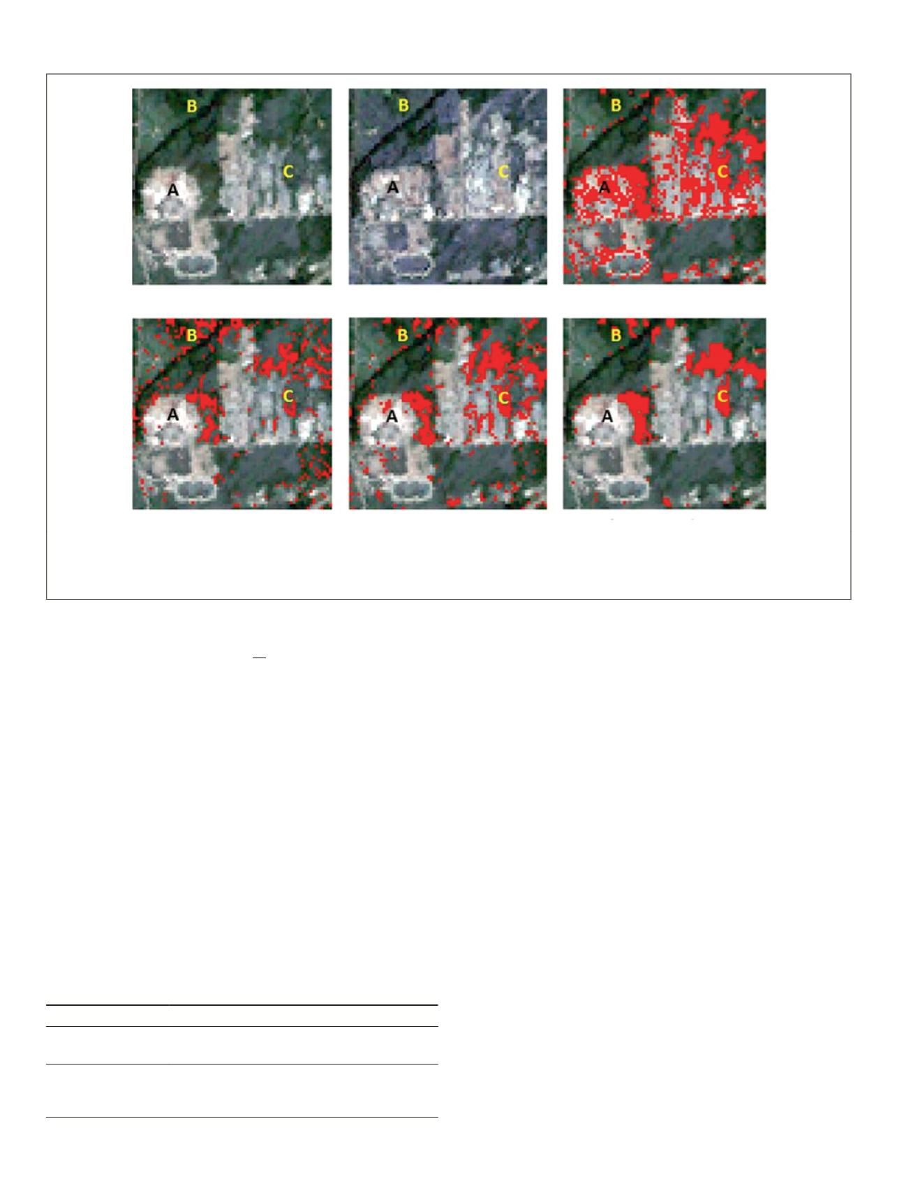
Plate 1. Examples of detection results for a small subset from steps in the proposed procedure: (a) the subset image acquired in 1991,
(b) the subset images acquired and 2001, (c) the detection result from thresholding the luminance band, (d) the detection result from
thresholding the saturation band, (e) the detection result after Bayes fusion of thresholding results in (c) and (d), and (f) the detection
result after MRF smoothing the results in (e). Changed pixels are highlighted as red.
T
able
1. G
rouping
S
trategy
for
F
inal
C
hange
-D
etection
M
ap
based
on
the
P
rior
A
ssumption
that
the
C
hange
only
O
ccurs when
B
oth
S
aturation
A
nd
L
uminance
C
hange
Subclass Names
“Change class”:
l
1
(
ω
pc
(
lu
),
ω
pc
(
sa
)),
l
2
(
ω
nc
(
lu
),
ω
pc
(
sa
)),
l
3
(
ω
pc
(
lu
),
ω
nc
(
sa
)),
l
4
(
ω
nc
(
lu
),
ω
nc
(
sa
))
“No-change class”:
l
5
(
ω
uc
(
lu
),
ω
pc
(
sa
)),
l
6
(
ω
uc
(
lu
),
ω
nc
(
sa
)),
l
7
(
ω
pc
(
lu
),
ω
uc
(
sa
)),
l
8
(
ω
nc
(
lu
),
ω
uc
(
sa
)),
l
7
(
ω
uc
(
lu
),
ω
uc
(
sa
))
640
August 2015
PHOTOGRAMMETRIC ENGINEERING & REMOTE SENSING


