time
values are used to apply rate parameters within a
CU
.
Now assume a
CU
for which the sensor errors significantly
vary throughout (perhaps due to a longer collection time or
greater aircraft dynamics). One set of
CU
-wide adjustable pa-
rameters may not be sufficient to capture the higher-frequency
errors for the entire
CU
. However, a set of
CU
-wide sensor
adjustable parameters combined with multiple sets of
sub-
CU
adjustable parameters, distributed throughout the
CU
by time
and associated with unique timestamps, could be applied.
The higher-frequency errors not captured by the
CU
-wide
adjustable parameters could be modeled by interpolating
between the sub-
CU
adjustable parameters. In Sensor-Space
ULEM
, these sub-
CU
adjustable parameters and their associated
covariances are defined as
posts
.
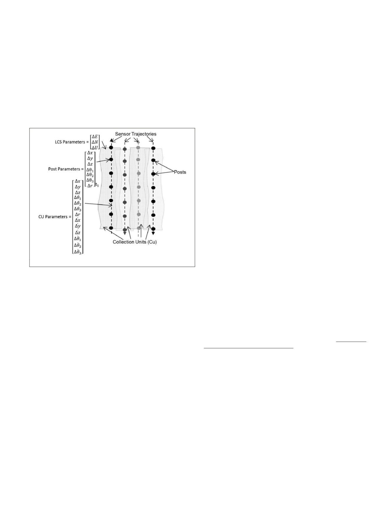
Figure 3. Sensor-Space
ulem
Adjustable Parameters.
Figure 3 illustrates the Sensor-Space
ULEM
adjustable
parameters for several passes of a lidar collection. Note that
the posts are illustrated as being along the trajectories of the
passes. This is not to imply that posts only apply to lidar
data that are
spatially
proximate. Posts are associated with a
particular epoch in time, and a post’s information will have
its greatest effect on lidar data that are
temporally
proximate.
The post parameters (based on the Sensor-Space
ULEM
general
adjustable parameters) are provided below for each
CU
i
and
post
j
:
• Δ
x
ij
,
Δ
y
ij
,
Δ
z
ij
:
PCS
positional offsets
• θ
1
ij
,
θ
2
ij
,
θ
3
ij
:
PCS
angular offsets
• Δ
r
ij
: range offsets
This set of parameters consisting of
CU
parameters,
LCS
pa-
rameters, and post parameters represent the
true
parameters
that are adjusted and solved during a
ULEM
adjustment.
Projective Model
The Sensor-Space
ULEM
projective model describes the relation-
ship among the range, sensor position, sensor orientation, and a
ground point. The projective model is shown in Equation 7:
x
y
z
x
y
z
M
r
=
+
S
S
S
L R|
0
0
(7)
In this model, [
x,y,z
]
T
represents a point in the point cloud
in the
LCS
. The sensor position, again in the
LCS
, is repre-
sented by [
x
S
, y
S
, z
S
]
T
. The rotation from the
RCS
to the
LCS
is
represented by
M
L|R
. Finally, the vector [0,0,
r
]
T
represents the
range vector from the sensor to the ground point in the
RCS
.
The
M
L|R
rotation matrix is defined by the rotation from the
RCS
to the
PCS
,
M
P|R
, and the rotation from the
PCS
to the
LCS
,
M
L|P
. This relationship is shown in Equation 8:
M
L|R
=
M
L|P
M
P|R
(8)
Stochastic / Adjustment Model
The Sensor-Space
ULEM
Stochastic/Adjustment Model,
detailed in Equation 9, is a modification of the
ULEM
Projec-
tive Model which designates the
ULEM
adjustable parameters
having probabilistic (stochastic) properties associated with
them. This model is necessary for both error propagation and
data adjustment. In order to form the Stochastic/Adjustment
Model, the
ULEM
projective model (Equation 7) is expanded
to include a series of adjustable parameters, all of which have
initial values of zero. Note that the relationship in Equation 8
was used to decompose the
M
L|R
matrix.
|
|
x
y
z
x
y
z
E
N
U
M
x
adj
=
+
+
S
S
S
L P
Δ
Δ
Δ
Δ
Δ
|
y
z
M M M M M
r r
Δ
Δ
θ θ θ
+
+
L P
P R
3 2 1
0
0
(9)
For
ULEM
, three distinct, and seven general adjustable
parameters have been identified. First, are the three distinct
coordinate translations (
Δ
E,
Δ
N,
Δ
U
) which provide adjust-
ments to the sensor position in the
LCS
. The general adjust-
able parameters include three translations (
Δ
x,
Δ
y,
Δ
z
) which
provide adjustments to the sensor position in the
PCS
, a range
bias (
Δ
r
), and three rotation parameters,
θ
1
,
θ
2
,
θ
3
(sequential
rotations about the
PCS
X
p
, Y
p
, Z
p
axes, respectively).
The general adjustable parameters in Equation 9 (
Δ
x,
Δ
y,
Δ
z,
θ
1
,
θ
2
,
θ
3
,
Δ
r
) may be
aggregates
of multiple contributors,
depending on which parameterization is implemented. Thus,
the true adjustable parameters, as discussed in the Param-
eterization Section above, are the
contributors
to the general
parameters shown in Equation 9. That is, a
ULEM
adjustment
consists of solving for corrections to these true (contributor)
parameters rather than the general (aggregate) values.
Since post parameters are temporally distributed within
a given
CU
i
, their contribution to the adjustment of a lidar
point will depend on the timestamp of that lidar point. Spe-
cifically, the contribution from the posts will be an interpo-
lated value from among all posts
j
within
CU
i
, which for the
Δ
x
parameter is designated
Δ
x
posts
, and similarly for the other
parameters.
Equation 10 provides all the possible contributors for each
of the aggregate adjustable parameters, for
CU
i
, with the “dot”
superscript indicating a rate parameter. Note that in practice
some subset of these may be used. Testing to date has gener-
ally involved parameterizations involving the
CU
offsets and
post contributions. The rate terms have typically not been
used, but including them in the model provides additional
flexibility for future implementers.
Δ
x
=
Δ
x
posts
+
Δ
x
i
+
Δ
·
x
i
dt
Δ
y
=
Δ
y
posts
+
Δ
y
i
+
Δ
·
y
i
dt
Δ
z
=
Δ
z
posts
+
Δ
z
i
+
Δ
·
z
i
dt
θ
1
=
θ
1
posts
+
θ
1
i
+
θ ·
1
i
dt
(10)
θ
2
=
θ
2
posts
+
θ
2
i
+
θ ·
2
i
dt
θ
3
=
θ
3
posts
+
θ
3
i
+
θ ·
3
i
dt
Δ
r
=
Δ
r
posts
+
Δ
r
i
+
Δ
·
r
i
dt
The
dt
term is a normalized time difference between the lidar
point’s timestamp,
t
, and the reference timestamp,
t
ref
, for the
CU
.
dt
= 2(
t
–
t
ref
)/(
t
CU end
–
t
CU start
), where the reference time-
stamp (
t
ref
= (
t
CU end
+
t
CU start
)/2) is the temporal midpoint of the
PHOTOGRAMMETRIC ENGINEERING & REMOTE SENSING
July 2015
549


