CU
based on the
CU
starting time (
t
CU start
) and
the
CU
ending time (
t
CU end
). Thus,
dt
= (2
t
–
t
CU end
–
t
CU start
)/(
t
CU end
–
t
CU start
).
After adjustment, if the solved parameters
are not applied to the points in the dataset,
the parameters can be stored for subsequent
use. However, it is important to note that if
the solved parameters from an adjustment
are applied to a Sensor-Space
ULEM
dataset,
and that dataset will remain in the Sensor-
Space
ULEM
implementation, then the trajec-
tory data [
x
S
,
y
S
,
z
S
]
t
must be updated using
the solved
LCS
translation parameters [
Δ
E
,
Δ
N
,
Δ
U
]
t
, and the aggregate
PCS
translation
parameters [
Δ
x
,
Δ
y
,
Δ
z
]
t
rotated to the
LCS
coordinate system using
M
L|P
. This is neces-
sary to ensure that the trajectory stored in
the point file is consistent with the updated
point locations for future range and
LOS
cal-
culations. The updated trajectory values are
calculated using Equation 11.
x
y
z
x
y
z
E
N
U
updated
S
S
S
S
S
S
=
+
+
Δ
Δ
Δ
M
x
y
z
L P|
Δ
Δ
Δ
(11)
Covariance Storage and Modeling
If employing the direct storage method, the upper-diagonal
entries of the full covariance matrix for adjustable param-
eters is stored in the
ULEM
metadata. When using the indirect
method, only the block-diagonal covariance entries of the full
covariance matrix are stored. The correlations and cross-cor-
relations are then modeled using the
SPDCF
, the parameters for
which are stored in the
ULEM
metadata. An example forma-
tion of an indirectly-stored full-covariance matrix is shown in
Equation 12, with
Σ
the full covariance matrix,
Σ
11
,
Σ
22
, …,
Σ
nn
the block-diagonal adjustable parameter covariance matrices
for
n
CUs,
Σ
ij
a cross-covariance term between CUs and
ρ
the
modeled correlation coefficient.
Σ
Σ Σ
Σ
Σ
Σ
Σ
ρ
=
=
11 12
1
22
2
n
n
nn
sym
SPDCF spdcf
.
(
)
/
/
parameters
ij
ii
jj
T
Σ ρΣ Σ
=
1 2 2
(12)
A similar approach is used to model the covariance be-
tween posts. Additional details on
ULEM
storage can be found
in the
ULEM
Implementation and Exploitation document.
(
NGA
, 2013)
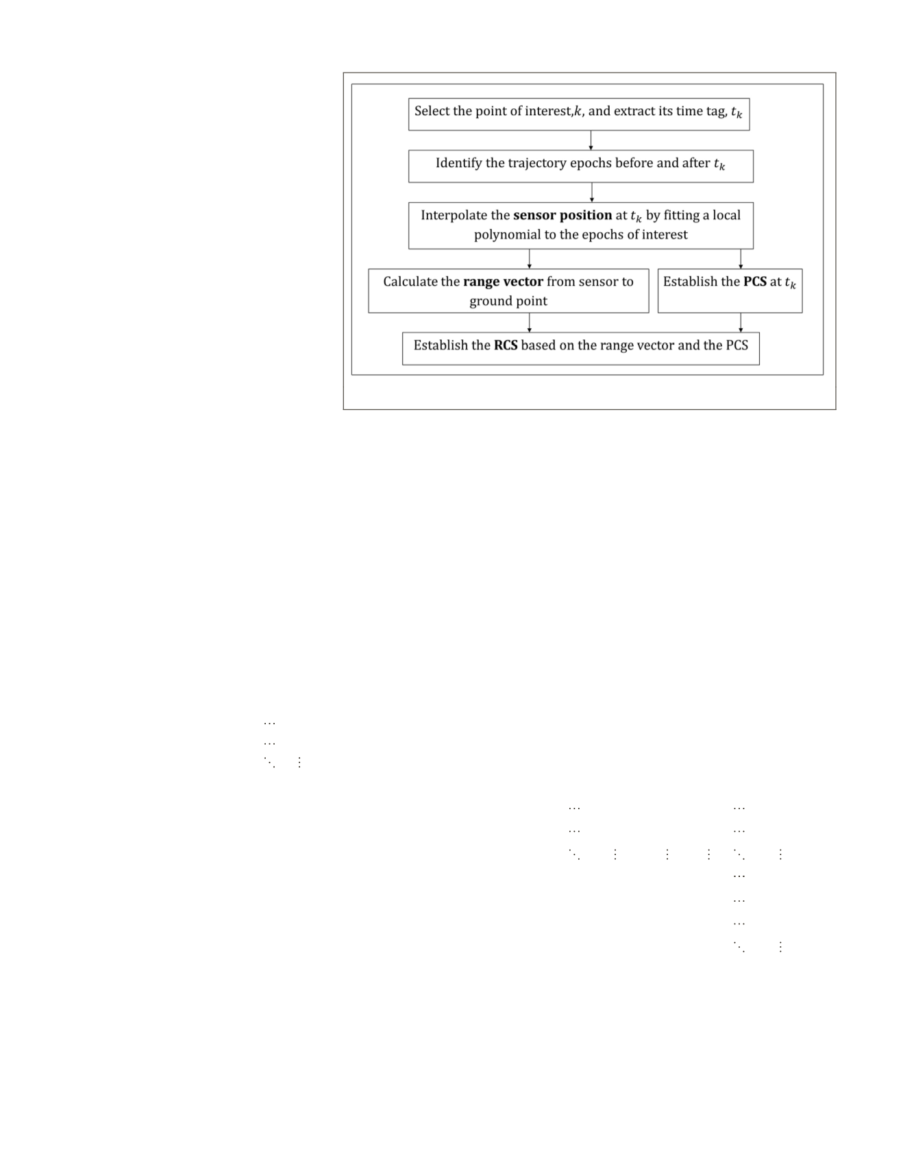
Exploitation
Before relating the details of exploitation, it is necessary to
describe what actually happens when one mensurates a point
in a lidar dataset containing Sensor-Space
ULEM
. This process
is described at a high level in Figure 4. The values obtained
after point mensuration include sensor position, the range
vector, and instantiations of the
PCS
and the
RCS
, all of which
are needed in the Stochastic / Adjustment Model.
One of the primary requirements for precise geoposi-
tioning is the use of error propagation to obtain predicted
uncertainties in a system, which for many systems is accom-
plished within the
CSM
construct (Rodarmel et al., 2011). As
previously discussed,
ULEM
is developed to be compatible
with
CSM
; however lidar modeling has yet to be fully incorpo-
rated into the
CSM
standard. Towards this goal, some changes
have been proposed to the
CSM
standard, including the ad-
dition of methods amenable to lidar exploitation. One of the
proposed methods is
modelToGround()
.
The modelToGround() method is an application of the
ULEM
adjustment model (Equation 9) followed by a coordi-
nate conversion to Earth-Centered-Earth-Fixed (
ECEF
) Carte-
sian coordinates. The “model” in modelToGround() refers to
model points
, which are lidar points in their native format
in the point cloud (e.g.,
UTM
), having coordinates defined as
model coordinates
. Optional mensuration-error covariance for
the model coordinates can be included as input to modelTo-
Ground(), which will enable ground covariance information
as additional output. The following example describes the
calculations needed to obtain the covariance of the output
ground point from modelToGround(). The example configura-
tion consists of two
CU
s, with the first
CU
having
n
1
posts and
the second
CU
having
n
2
posts. First, the covariance matrix of
the adjustable parameters,
Σ
a
, is formed for all the parameters
in the configuration chosen for the dataset as in Equation 13.
,
Σ
Σ Σ
Σ
Σ
Σ
a
=
CU
CU
P
P P
P
n
n
1
12
11
11 1 1
1 1
0
0
0
0
0 0
0
0 0
0
0
0
2
21
21 2 2
2 2
.
,
Σ
Σ
Σ
Σ
CU
P
P P
P
n
n
sym
(13)
In Equation 13,
Σ
CU
i
represents the covariance of the
i
th
CU
parameters and
Σ
P
ij
represents the covariance of post param-
eters for post
j
in
CU
i
. The component submatrices within are
detailed in Equation 14. In this example, the
CU
adjustable
parameters are offsets (
Δ
x
,
Δ
y
,
Δ
z
,
Δ
r
) and rates (
Δ
·
x
,
Δ
·
y
,
Δ
·
z
).
Correlations are modeled within three separate groups, the
first one containing (
Δ
x
,
Δ
y
,
Δ
·
x
,
Δ
·
y
), the next one containing
Figure 4.
ulem
Mensuration of a point.
550
July 2015
PHOTOGRAMMETRIC ENGINEERING & REMOTE SENSING


