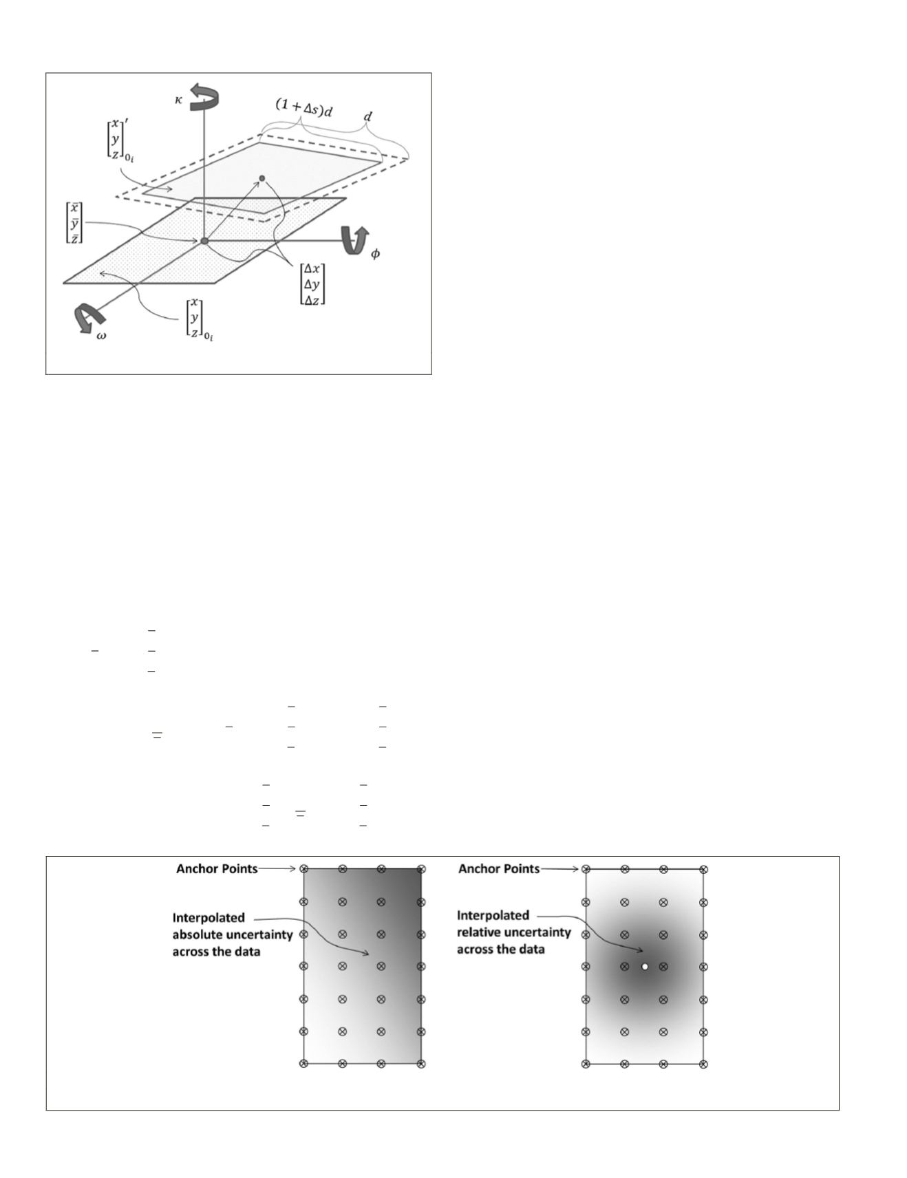
Figure 5. 3D Conformal (3DC) Coordinate Transformation.
In Equation 18, [
xy z
]
T
0
represents normalized and re-cen-
tered (to the
CU
centroid) model-space coordinates prior to
transformation. These are formed using Equation 19, where
[
xy z
]
T
are the original model-space coordinates, [
x
–
y
–
z
– ]
T
are
the re-centering values, and
s
– is a normalizing scale factor.
The re-centering values are the coordinates of the centroid
of the
CU
, and the scale factor is such that it normalizes all
re-centered point coordinates with respect to the longest dis-
tance between points in the
CU
. All of these values are stored
and carried in the
ULEM
metadata. After the transformation is
applied, the result, ([
xy z
]
0
´
)
T
, must be multiplied by 1/
s
– , and
the re-centering offset must be removed by adding [
x
–
y
–
z
– ]
T
to
obtain the final adjusted coordinates ([
xy z
]
´
)
T
. The full trans-
formation equation is shown in Equation 20a, and an equiva-
lent simplified version (after a cancellation) in Equation 20b.
x
y
z
s
x
y
z
x
y
z
=
−
0
(19)
x
y
z
f
x
y
z
s
s Ms
x
y
z
i
i
=
= +
'
(
)
1
1
−
+
i
x
y
z
x
y
z
+
x
y
z
(20a)
x
y
z
f
x
y
z
s M
x
y
z
i
i
=
= +
'
(
)
1
−
+
+
i
x
y
z
s
x
y
z
x
y
z
1
(20b)
The covariance matrix associated with the 3DC transforma-
tion adjustable parameters (
Σ
3
DC
l
), for some
CU
, can be formed
as shown in Equation 21. In this equation,
ω
,
ϕ
, and
κ
are se-
quential rotations about the re-centered model-space
x, y,
and
z
axes, respectively, and are those used to form
M
of Equation
18. When not all of the 3DC transformation parameters are
used, the covariance matrix consists of a subset of the appro-
priate elements of Equation 21.
φ
φ
κ
σ σ
κ
Σ
σ σ
σ
σ
σ
σ
σ
σ
σ
σ
σ
σ
ω
κ
ω
3
2
2
DC
l
x
x y
x z
x
x
x
x s
y
y z
y
y
y
=
φ
φ
ω
κ
ω ω
φ
ωκ
ω
σ
σ
σ
σ
σ
σ
σ σ
σ
σ
σ
y s
z
z
z
z
z s
s
2
2
2
φ
φ
s
s
s
sym
.
σ σ
σ
κ
κ
2
2
(21)
If the 3
DC
model cannot accurately represent a dataset, the
user may implement the Anchor Point model. This model is
based on the storage of covariance data at
anchor points
that
reflect the local phenomena in the data. These anchor points
are at specified locations within the point cloud, each with
an associated error covariance. Additionally, the correlation
among the errors associated with the anchor points is stored,
enabling the formation of their full covariance matrix.
The full anchor point covariance matrix characterizes the
overall relationships among uncertainties at their locations.
When only anchor points are implemented, the absolute
uncertainty of any point and the relative uncertainty of any
point pair can be estimated by propagating the anchor point
covariance to ground-space using partial derivatives with
respect to the anchor point parameters. Figure 6 is a graphi-
cal illustration of interpolated absolute (6a) and relative (6b)
uncertainty. In Figure 6a, the shading of each anchor point
represents the variance at their location and the shading
across the dataset area represents the interpolated variance.
In Figure 6b, the anchor point shading represents the relative
variance between the anchor points and the point located in
the center, and the shading across the dataset represents the
interpolated relative variance with respect to the center point,
where darker shading represents lower relative variance. The
anchor point adjustable parameters in the Ground-Space
ULEM
are translations (
Δ
x
,
Δ
y
,
Δ
z
) associated with anchor point
locations. Anchor points should be distributed throughout
a point cloud area in such a way that the interpolation can
sufficiently capture error phenomena and the interpolation
method can operate adequately.
(a) (b)
Figure 6. Interpolation of Uncertainties using Anchor Points.
552
July 2015
PHOTOGRAMMETRIC ENGINEERING & REMOTE SENSING


