PE&RS July 2015 - page 579

bands 4 and 5, OLI bands 5 and 6). These three layers, along
with other ancillary data, are used by the mapping analysts to
manually filter desired change from spurious noise or unde-
sired change. An example of undesired change would be agri-
cultural areas that are masked out of the MIICA biomass change
products using the Cropland Data Layer available from the
National Agricultural Statistics Service (Boryan et al., 2011).
The dNBR data are further used to estimate the severity of dis-
turbances. For each dNBR image, the global mean and standard
deviation (STDEV) are computed. The data are then classified
into four severity classes where the dNBR values are: greater
than 1 stdev above the global mean, within 1 stdev above the
global mean, within 1 stdev below the global mean, and all
other values. For each disturbance date, the maximum sever-
ity class of the two dNBR images corresponding to that date
is used as the severity estimate for that date. For example,
for 2011 day 175 severity, the 2010 day 175 to 2011 day 175
dNBR, and the 2011 day 175 to 2012 day 175 dNBR images
are considered. This process is repeated using two and three
stdevs resulting in three severity estimates per date. These es-
timates are then used by the analysts to assign severity values
to each MIICA-detected disturbance, both fire and non-fire.
Browse
The last step in the process of stacking and tiling is to create
full resolution browse images of the resulting tile, as well as
reduced resolution thumbnails. Satellite imagery is presented
as a false color TM composite with bands 7, 5, and 3, and is
stored in JPEG format for easy viewing in a web browser. Mask
imagery are color-mapped in both full and reduced resolu-
tion and are stored in PNG format. The browse imagery is used
for quick assessments of image quality and general refer-
ence where the full pixel data are not needed. They are also
integrated into a web-based quality assurance and progress
tracking system used by the LANDFIRE analysts during produc-
tion processing.
Results
Scene Processing
A total of 20,489 images were processed to create the CONUS
tiles: 9,870 TM, 5,109 ETM+, and 5,510 OLI . Most scenes were
split among multiple tiles. There were 47,038 partial scenes
among the 98 tiles: 22,683 TM, 11,672 ETM+, and 12,683 OLI.
Each scene was used in an average of two to three tiles. The
average number of scenes used to create each tile varied from
54 to 68 (Table 2). Each tile was manually reviewed for quality
prior to completion. Tiles that were found to have excessive
cloud cover remaining, data gaps due to incomplete input
scene lists, incorrectly clipped bumper mode edges, or poor
geometric registration were reprocessed to address these issues.
Geometric registration of Landsat data is generally well
characterized for all LPGS-processed imagery. However, sev-
eral anomalous ETM+ scenes were discovered in the course
of manual review of the output tiles. The scenes in ques-
tion had been processed to Level 1T and therefore should
have been registered within ±30 m according to the product
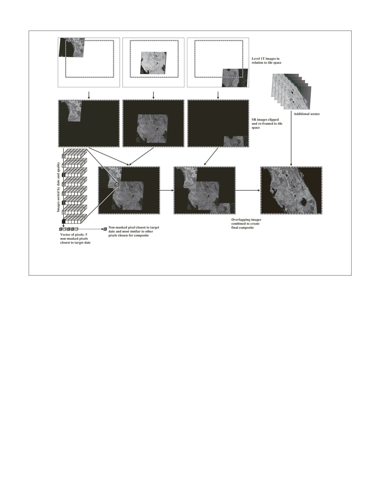
Figure 3. Overview of tiled composite process. Level 1T images are clipped and re-framed to tile space. Overlapping images are
sorted by date and image quality. Vectors of pixels are extracted at each pixel location containing a maximum of five non-masked
pixels closest to the target date. One pixel is selected from the vector based on distance to target date and similarity to other pixels
in the vector and is used to populate the final composite tile.
PHOTOGRAMMETRIC ENGINEERING & REMOTE SENSING July 2015 579