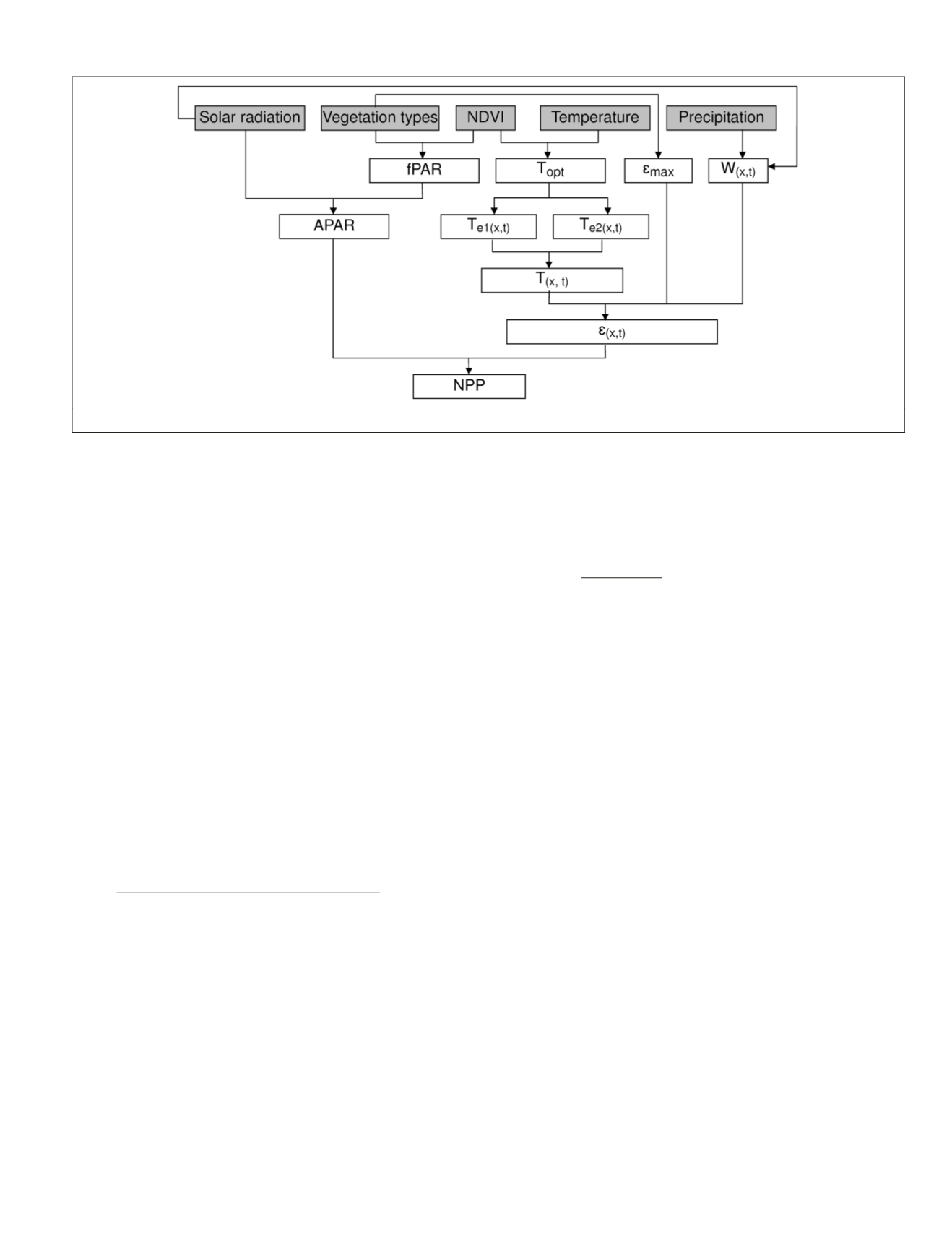
The actual light use efficiency (
ε
x,t
) is generally affected by
the suitability of temperature and availability of water for a
given location and month-based time (x, t), and is also con-
sidered to be smaller than the maximum light use efficiency
of vegetation (
ε
max
). So, the actual light use efficiency (
ε
x,t
) can
be calculated using Equation 4 by multiplying the index of
water availability (W
x,t
) and the index of temperature suit-
ability (T
x,t
) and the scalar
ε
max
(gC MJ
-1
). According to Zhu et
al. (2006), the
ε
max
of the vegetation types were given as 0.589,
0.542, 0.485, 0.310, and 0.000 for forest, steppe, desert steppe,
desert, and water, respectively.
In Equation 4, T
e1
and T
e2
account for the effects of temper-
ature stress on plant growth. T
e1
is used to reflect the empiri-
cal observation that plants in very cold habitats typically have
low growth rates and high root biomass, potentially imposing
large respiratory costs. In contrast plants in very hot environ-
ments may have high growth rates while the efficiency of
light utilization could be impacted by high rates of respiration
(Ryan, 1991). T
e1
expressed in Equation 5 is a function of op-
timum temperature (T
opt
, that is defined as the air temperature
for the month when the
NDVI
reaches its maximum in a year
)
and varies spatially but not temporally.
ε
(x,t)
= T
(x,t)
× W
(x,t)
×
ε
max
= T
e1(x,t)
× T
e2(x,t)
× W
(x,t)
×
ε
max
(4)
T
e1(x)
= 0.8 + 0.02T
opt(x)
– 0.0005(T
opt(x)
)
2
(5)
T
e2(x)
=
1.1814
{1+e
[0.2(–T
opt(x)
–10–T
air(x,t)
)]
}×{1+e
[0.3(–T
opt(x)
–10+T
air(x,t)
)]
}
(6)
For a T
opt
of 0°C, T
e1
equals 0.8. The scalar rises paraboli-
cally to 1.0 at 20°C and then falls to 0.8 at 40°C. It varies only
between 0.8 and 1. This is because virtually all terrestrial
ecosystems have growing season temperatures between 0°C
and 40°C. For mean monthly temperatures of below –10°C, T
e1
is set to zero. T
e2
reflects the consideration that the efficiency
of light utilization should be reduced when plants are grow-
ing at temperatures at variance with their optimum. This has
an asymmetric bell shape that falls off more quickly at high
and low temperatures. In Equation 6, T
air
is the mean monthly
air temperature. T
e2
equals 1 when T
air
= T
opt
and it falls to half
its value at T
opt
at the two conditions, i.e., T
air
is 10°C above or
T
air
is 13°C below T
opt
.
The index of water availability for a given location grid
x time t (W
x,t
) can be determined using Equation 7 in which
E
p(x,t)
and E
(x,t)
represent the potential evapotranspiration and
the estimated evapotranspiration and were calculated using
Equation 8 (Yu
et al
., 2009). W
(x,t)
varies from 0.5 in very arid
ecosystems to 1 in very wet ecosystems. E
po(x,t)
and E
(x,t)
in
Equation 8 were calculated using the methods of Thornth-
waite (1948) and Yu
et al
. (2009), respectively.
W
(x,t)
= 0.5 +
0.5 × 0.5E
(x,t)
E
p(x,t)
(7)
E
p(x,t)
= E
(x,t)
+ 0.5E
po(x,t)
, 0°C
≤
T
air
≤
26°C
(8)
Statistical Analysis of the Changes of NPP Changes
In this study, the temporal-spatial variation of the
NPP
involves three independent variables (Vegetation types or
VT, time-monthly or tMo, and time-yearly or tYr). Factorial
experiment design offers a better efficiency in the study of the
main effects of the multiple factors (i.e., variables) and at the
same time the interaction effect between factors. A fixed mod-
el-based three-way factorial design was applied to account
for the full component of all possible variable combinations
including the main and interaction effects as shown in Equa-
tion 9 where the coefficients
β
i
,
β
ij
, and
β
ijk
represent the effects
of the three main variable, the three two-variable interaction,
and the one three-variable interaction on the dependent vari-
able Y, the determined yearly-monthly
NPP
(gC m
–2
mo
–1
).
Y
=
β
0
+
β
1
X
1
+
β
2
X
2
+
β
3
X
3
+
β
12
X
1
X
2
+
β
13
X
1
X
3
+
β
23
X
2
X
3
+
β
123
X
1
X
2
X
3
+
ε
(9)
In the
ANOVA
analysis, an effect is said to be significant if
its coefficient is with a probability less than or equal to the
significant probability 0.05. This indicates that the
NPP
chang-
es significantly among the treatments (also named levels) of
a factor or 2- to 3-factor interaction. A moderate conservative
post hoc test, Duncan’s new multiple range test is then ap-
plied for interpreting multiple comparisons. Since the num-
ber of treatments of the factors is 4, 7, and 5 for VT, tMo, and
tYr, respectively, Duncan’s method can provide a reasonable
determination of the difference between any two treatments’
mean (
μ
i
=
μ
j
for all
i
≠
j
) due to the nature of the significance
level protection. Regression analysis was applied to examine
the relationship between the
NPP
of terrestrial ecosystems and
the climatic factors and to derive the models for predicting
the percentage area of
NPP
increment in growing season.
Figure 1. Data flow in
npp
prediction.
PHOTOGRAMMETRIC ENGINEERING & REMOTE SENSING
July 2015
589


