I
w x b
i
n
i i
=
+
=
∑
1
(5)
where
I
correspond to the node value,
n
is the source space di-
mension or number of input data (
x
i
),
w
i
is the weight of an input
signal, and
b
is the bias associated with the target scalar (node).
The model parameters and bias term for each node were
then optimized using a network activation function, and then
these optimal model parameters and biases minimized the er-
ror between the desired output and the actual one for all train-
ing patterns. Finally, the output layer provided the response of
the neural network to the pattern vector submitted in the input
layer (Mas and Flores, 2008). In this research, the multitem-
poral
ALOS
PALSAR
backscatter values were used as a source to
estimate the
AGB
as a target space, and the number of hidden
layers and iterations were set to 2 and 1000, respectively.
The Support Vector Machine is a nonlinear kernel-based
technique for classification, regression, and function approxima-
tion in the multidimensional space of the data (Mountrakis
et
al.
, 2011). The
SVR
function for biomass estimation is de ned as:
AGB k x x b
i
n
i
i
=
+
=
∑
1
α
( ; )
(6)
where
k
(
x
i
;
x
) is a kernel function with the training vector
x
i
,
and
α
is Lagrange multiplier.
A radial basis function (
RBF
) kernel is typically chosen as a
kernel function:
K x x
x x
i
i
,
exp
(
)
=
−
(
)
2
2
σ
(7)
where
σ
is a scale parameter chosen based on the training
data, and a unit vector could be concatenated with kernels
as the intercept (further details can be found in Rabe
et al.
,
2009).
Although
SVR
parameters are specified to be fixed for any
predefined numbers, they should be defined using a cross
validation approach. Further, because
SVR
is very sensitive
to parameters, it is very important to define them properly.
Hence, the accuracy of the
SVR
model can be significantly
improved by choosing the correct bias for the parameters. As
previously stated, the input vectors for
MLPNN
,
SVR
, and
MVRVR
in this paper are the multitemporal
ALOS
PALSAR
backscatter
values.
Estimation of AGB Using the MVRVR Method
As described in the Introduction, in this study we applied
an
MVRVR
model to estimate the forest
AGB
. It is important to
mention that
MVRVR
is a multivariate regression approach,
which means that a
MVRVR
model can also be used to find
the non-linear mapping function among input (source) and
output (target) data, even if their (input and output) dimen-
sions are greater than one. The simplified MRVM model for
the target point, for example
AGB
values, with one dimension
is de ned as:
AGB
=
W
Φ
(
x
)+
ε
(8)
where
W
is the weight matrix,
ε
is a zero-mean Gaussian noise
with a diagonal covariance matrix,
S
=
diag
[
σ
1
2
,σ
σ
2
2
,〖…,σ
σ
P
2
], and
Φ
(
x
) is a basis vector of kernel function.
In relation to the scalar values of
AGB
, the generalized (mul-
tivariate) form of the
MVRVR
approach is redundant, and thus
the formulations are developed using only a single mapping
function. In the Bayesian framework, a zero-mean Gaussian
prior is considered for the weight matrix to induce scarcity, as:
p W
w
i
n
j
m
i j
j
( |A
| )
)
(
,
,
=
= =
−
∏∏
1 1
2
0
α
(9)
where
m
is the target space dimension or the output data, and
A
is a hyperparameter matrix. In this case, the target space
dimension (
AGB
values) is equal to one.
The mapping function parameters are weight, covariance,
and the hyperparameter matrix. A possible distribution of the
mapping function is formulated as:
p AGB W AGB W x
i
i
n
i
| S
(
|
S
,
.
, )
(
)
=
( )
=
∏
1
Φ
(10)
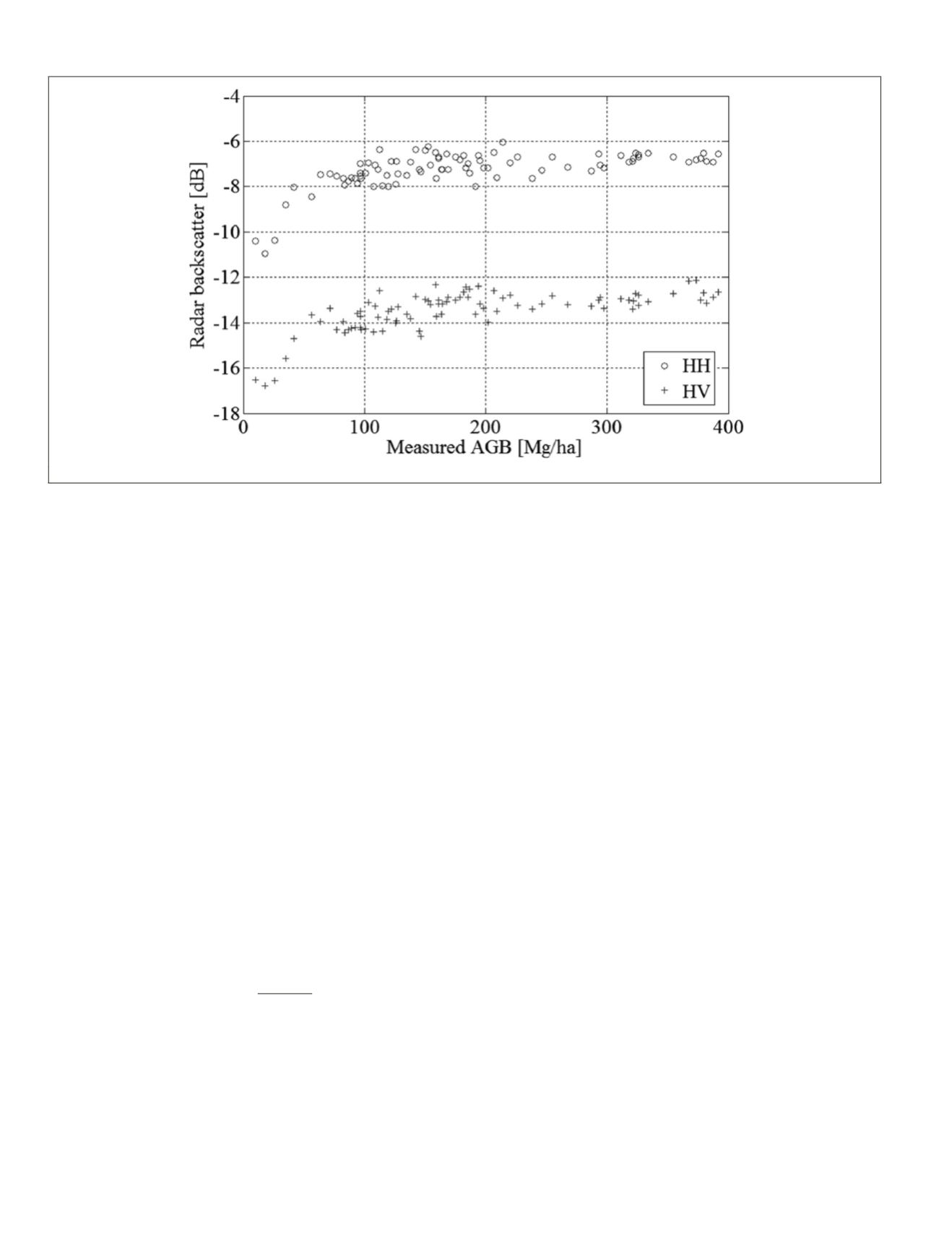
Figure 1. Temporal average of 110 radar backscatters in HH and HV polarizations versus field AGB.
44
January 2016
PHOTOGRAMMETRIC ENGINEERING & REMOTE SENSING


