Sensor Topology
Most of modern LiDAR sensors offer an intrinsic 2D topology
in raw acquisitions. However, this feature is rarely considered
in recent works. Namely, LiDAR points may obviously be or-
dered along scanlines, yielding the first dimension of the sensor
topology, linking each LiDAR pulse to the immediately preced-
ing and succeeding pulses within the same scanline. For most
LiDAR devices, one can also order the consecutive scanlines. It
amounts to considering a second dimension of the sensor topol-
ogy across the scanlines as it can be seen in Figure 2.
From Sensor Topology to Range Image
The sensor topology often varies with the type of LiDAR sen-
sor that is being used. 2D LiDAR sensors (i.e., featuring a sin-
gle simultaneous scanline acquisition) such as the one used
in (Paparoditis
et al.
, 2012) generally send an almost constant
number
H
of pulses per scanline (or per turn for 360 degree
2D lidars) where each pulse was emitted at a certain
θ
angle
value. Therefore, any measurement of the sensor might be or-
ganized in an image of size
W
×
H
, where W is the number of
consecutive scanlines and thus a temporal dimension. This is
illustrated in Figure 3 in which one can see how the 2D image
is spanned by the sensor topology. In this work, such images
are only built using the range measurement as pixel intensity,
later referred to as range images. Note that these range images
differ from typical range images (Kinect,
RGB-D
) as the origin
of acquisition is not the same for each pixel and the 3D direc-
tions of pixels are not regularly spaced along the image, but
warped by the orientation changes of the sensor trajectory.
3D LiDAR sensors are based on multiple simultaneous
scanline acquisitions (e.g.,
H
= 64 fibers) such as in the
MMS
proposed in (Geiger
et al
., 2013). Again, each scanline con-
tains the same number of points and each scanline may be
stacked horizontally to form the same type of structure, as il-
lustrated in Figure 4. Note that Figures 3 and 4 are simplified
for better understanding, but that realistic cases can be more
chaotic as discussed later in this section.
Whereas LiDAR pulses are emitted somewhat regularly,
many pulses yield no range measurements due, for instance,
to reflective surfaces, absorption or absence of target objects
(e.g., in the sky direction) or an ignored measurement when-
ever the measure is too uncertain. Therefore, the sensor topol-
ogy is only a relevant approximation for emitted pulses but
not for echo returns, such that the range image is sparse with
undefined values where the sensor measured no echoes (or
when further processing was performed on the acquisition,
leading to the removal of points having a too uncertain mea-
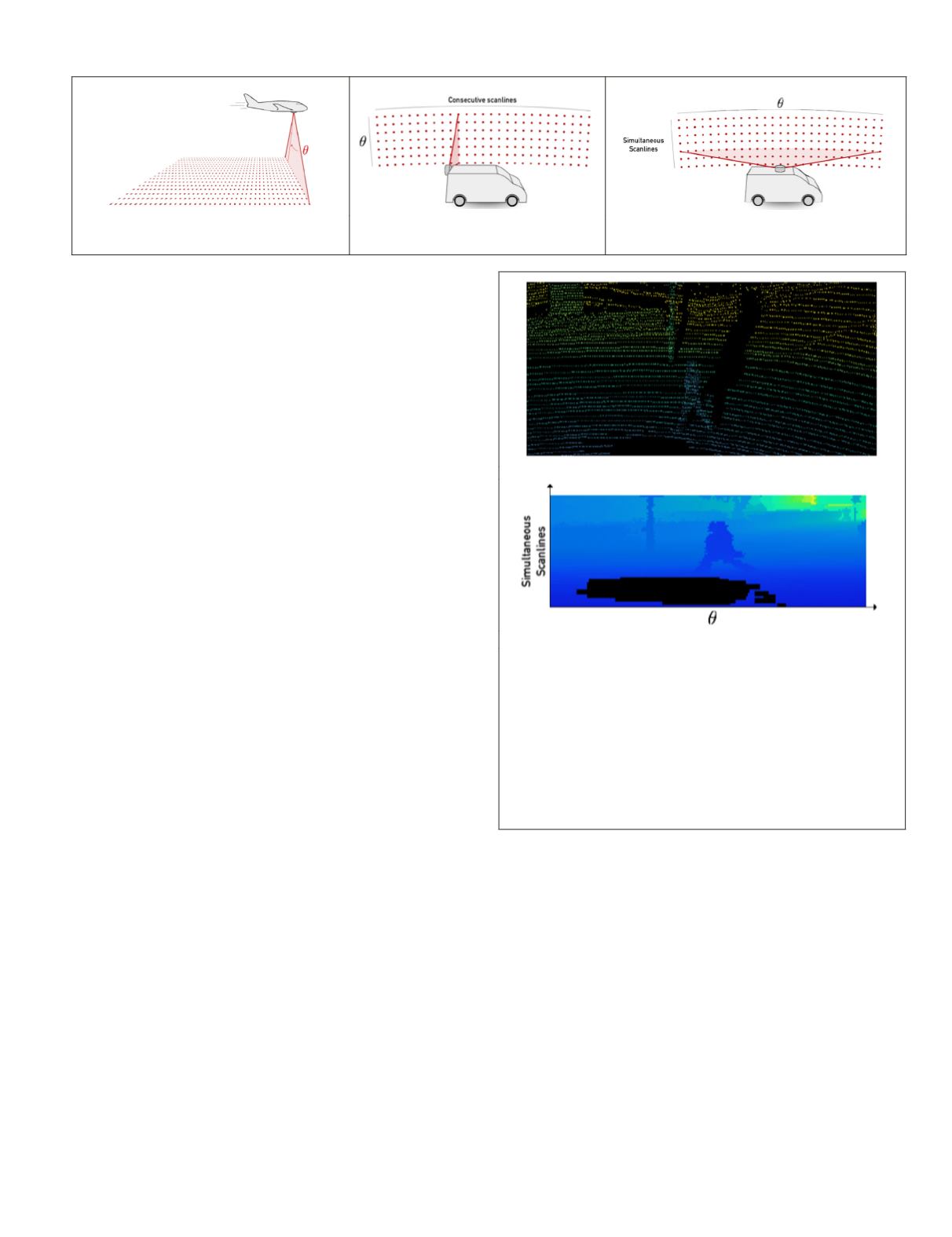
surements). This is illustrated in Figure 5b in which pulses
with no echoes appear in dark. Note that considering multi-
echo datasets as a multilayer depth image is beyond the scope
of this paper, which only considers first returns.
This 2D sensor topology encodes an implicit neighborhood
between LiDAR measurement pulses. Whereas the implicit
topology of pixels in optical images is supported by a regular
geometry of rays (shared origin and regular grid of directions
if geometric distortion is neglected), the proposed 2D sensor
topology for LiDAR point clouds is supported by the trajectory-
warped geometry of 3D rays. However, it readily provides, with
minimal effort, an approximation of the immediate 3D point
neighborhoods, especially if the sensor moves or turns slowly
compared to its sensing rate. We argue however that this is an
approximation.
We argue that most raw LiDAR datasets contain all the
information (scanline ordering, pulses with no echo, number
of points per turn, etc.) to enable the access to a well-defined
implicit sensor topology. However it sometimes occurs that
the dataset received further processing (points were reordered
or filtered, or pulses with no return were discarded) or that
the sensor does not acquire neighboring points consecutively.
Therefore, the sensor topology may then only be approxi-
mated using auxiliary point attributes (time,
θ
, fiber id…) and
guesses about acquisition settings (e.g., guessing approximate
∆
time or
∆
θ
values between successive pulse emissions).
Using this information, one can recreate the range map by
stacking points even if some points were discarded. Defining
a grid-like topology is a good approximation if the number
of pulses per scanline/per turn is close to an integer constant
with relatively stable rotation offsets between pulses.
Figure 2. Example of the intrinsic topo-
logy of a 2D
LiDAR
sensor built on a plane.
Figure 3. Example of 2D
LiDAR
sensor
and the related topology.
Figure 4. Example of 3D
LiDAR
sensor and the
related topology.
(a)
(b)
Figure 5. Example of a point cloud from the
KITTI
database
(Geiger et al., 2013) (a) turned into a range image (b). Note
that the dark area in (b) corresponds to pulses with no returns
is sufficient for most purposes, as it has the added advan-
tage of providing pulse neigh- borhoods that are reasonably
local both in terms of space and time, thus being robust to
misregistrations, and being very efficient to handle (constant
time access to neighbors). Moreover, as
LiDAR
sensor designs
evolve to higher sampling rates within and/or across scan-
lines, the sensor topology will better approximate spatio-tem-
poral neighborhoods, even in the case of mobile acquisitions.
PHOTOGRAMMETRIC ENGINEERING & REMOTE SENSING
June 2018
369


