in the projection of the depth of each pixel along the axis
formed by each corresponding point and the sensor origin. We
can see that the acquisition lines are properly retrieved after
removing the pedestrian. This result was generated in 4.9 sec-
onds using Matlab on a 2.7
GHz
processor. Note that a similar
analysis can be done on the results presented in Figure 1.
Dense Point Cloud
In this work, we aim at presenting a model that performs well on
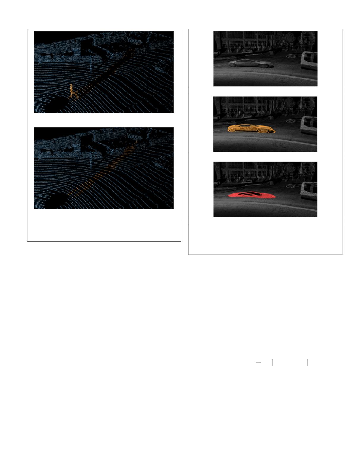
both sparse and dense data. Figure 14 shows a result of the dis-
occlusion of a car in a dense point cloud. This point cloud was
acquired using the Stereopolis-II system (Paparoditis
et al
., 2012)
and contains over 4.9 million points. In Figure 14a, the original
point cloud is displayed with the color based on the reflectance
of the points for a better understanding of the scene. Figure 14b
highlights the segmentation of the car using our model (with the
same parameters as in the Results and Analysis Section), dilated
to prevent aberrant points. Finally, Figure 14c depicts the result
of the disocclusion of the car using our method.
We can note that the car is perfectly removed from the
scene. It is replaced by the ground that could not have been
measured during the acquisition. Although the reconstruction
is satisfying, some gaps are left in the point cloud. Indeed,
in the data used for this example, pulses returned with large
deviation values were discarded. Therefore, the windows and
the roof of the car are not present in the point cloud before
and after the reconstruction as no data is available. We could
have added these no-return pulses in the inpainting mask as
well to reconstruct these holes as well.
Quantitative Analysis
To conclude this section, we perform a quantitative analy-
sis of our disocclusion model on the
KITTI
dataset. The
experiment consists in removing areas of various point clouds
in order to reconstruct them using our model. Therefore, the
original point clouds can serve as ground truth. Note that ar-
eas are removed while taking care that no objects are present
in those locations. Indeed, this test aims at showing how the
disocclusion step behaves when reconstructing backgrounds
of objects. The size of the removed areas corresponds to an
approximation of a pedestrian’s size at 8 meters from the sen-
sor in the range image (20 × 20px).
The test was done on 20 point clouds in which an area
was manually removed and then reconstructed. After that,
we computed the
MAE
(Mean Absolute Error) between the
ground truth and the reconstruction (where the occlusion was
simulated) using both Gaussian disocclusion and our model.
We recall that the
MAE
is expressed as follows:
MAE
u u
N
u i j u i j
i j
1 2
1
2
1
,
,
,
,
(
)
=
( )
−
( )
∈
∑
Ω
(5)
where
u
1
,
u
2
are images defined on
Ω
with
N
pixels where
each pixel intensity represents the depth value. Table 1 sums
up the result of our experiment. We can note that our method
provides a great improvement compared to the Gaussian
disocclusion, with an average
MAE
lower than 3 cm. These re-
sults are obtained on scenes where objects are located from 12
to 25 meters away from the sensor. The result obtained using
our method is very close to the sensor accuracy as mentioned
by the manufacturer ( ~– 2cm).
(a)
(b)
Figure 13. 3D representation of the disocclusion of the
pedestrian presented in Figure 12. (a) is the original mask
highlighted in 3D, (b) is the final reconstruction.
(a)
(b)
(c)
Figure 14. Result of the disocclusion on a car in a dense
point cloud. (a) is the original point cloud colorized with
the reflectance, (b) is the segmentation of the car highlighted
in orange, (c) is the result of the disocclusion. The car is
entirely removed and the road is correctly reconstructed.
PHOTOGRAMMETRIC ENGINEERING & REMOTE SENSING
June 2018
373


