Interest and Applications
The use of range images as the simplified representation of
a point cloud directly brings spatial structure to the point
cloud. Therefore, retrieving neighbors of a point, which was
formerly done using advanced data structures (Muja and
Lowe, 2014), is now a trivial operation and is given without
any ambiguities. This was proved to be very useful in applica-
tions such as remeshing, since faces can be directly associ-
ated to the grid structure of the range image. As shown in this
paper, considering a point cloud as a range image supported
by its implicit sensor topology enables the adaptation of the
many existing image processing approaches to LiDAR point
cloud processing (e.g., segmentation, disocclusion). More-
over, when optical data was acquired along with LiDAR point
clouds, the range image can be used for improving the point
cloud colorization and the texture registration on the point
cloud as the silhouettes present in the range image are likely
to be aligned with the gradients of optical images.
In the following sections, the LiDAR measurements,
equipped with this implicit 2D topology, are denoted as the
sparse range image
u
R
.
Application to Point Cloud Segmentation
In this section, a simple yet efficient segmentation technique
that takes advantage of the range image will be introduced.
Results will be presented and a quantitative analysis will be
performed to validate the model.
Range Histogram Segmentation Technique
We now propose a segmentation technique based on range
histograms. For the sake of simplicity, we assume that the
ground is relatively flat and we remove ground points, which
are identified by plane fitting.
Instead of segmenting the whole range image
u
R
directly,
we first split this image into
S
sub-windows
u
s
R
,
s
= 1 . . .
S
of
size
W
s
×
H
along the horizontal axis to prevent each sub-
window from representing several objects at the same range.
For each
u
s
R
, a depth histogram
h
s
of
B
bins is built. This
histogram is automatically segmented into
C
s
classes using
the
a-contrario
technique presented in Delon
et al
. (2007).
This technique presents the advantage of segmenting a 1D-
histogram without any prior assumption, e.g., the underlying
density function or the number of objects. Moreover, it aims
at segmenting the histogram following an accurate definition
of an admissible segmentation, preventing over- and under-
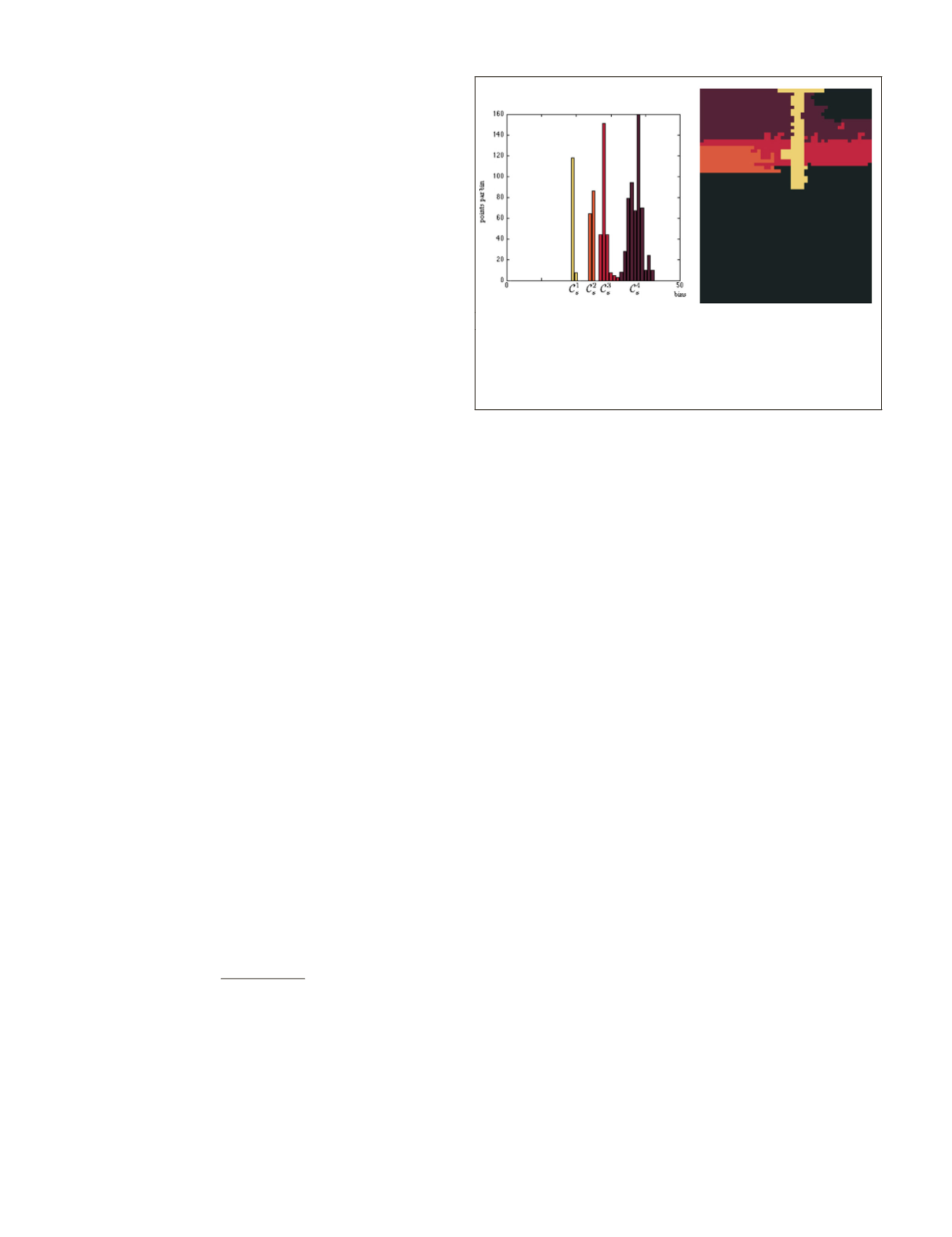
segmentation. An example of a segmented histogram is given
in Figure 6.
Once the histograms of successive sub-images have been
segmented, we merge together the corresponding classes by
checking the distance between each of their centroids in order
to obtain the final segmentation labels. Let us define the cen-
troid
C
s
i
of the i
th
class
C
i
s
in the histogram
h
s
of the sub-image
u
s
R
as follows:
C
b h b
h b
s
i
s
b C
s
b C
s
i
s
i
=
×
( )
( )
∈
∈
∑
∑
(1)
where
b
are all bins belonging to class
C
s
i
. The distance
between two classes
C
s
i
and
C
r
j
of two consecutive windows
r
and
s
can be defined as follows:
d
(
C
s
i
,
C
r
j
) = |
C
s
i
–
C
r
j
|
(2)
Finally, we can set a threshold such that if
d
(
C
s
i
,
C
r
j
)
≤
τ
,
classes
C
s
i
and
C
r
j
should be merged (e.g., they now share the
same label). If two classes of the same window are eligible
to be merged with the class of another window, then only
the one with lower depth should be merged. Results of this
segmentation procedure can be found in the next subsection.
The choice of
W
s
,
B
and
τ
mostly depends on the type of data
that is being treated (sparse or dense). For sparse point clouds
(few thousand points per turn),
B
has to remain small (e.g., 50)
whereas for dense point clouds (> 10
5
points per turn), this
value can be increased (e.g., 200). In practice, we found out
that good segmentations may be obtained on various kinds of
data by setting
W
s
= 0.5 ×
B
and
τ
= 0.2 ×
B
. Note that the win-
dows are not required to be overlapping in most cases, but for
very sparse point clouds, an overlap of 10 percent is enough to
achieve good segmentation. For example in our experiments
on the
KITTI
dataset (Geiger
et al
., 2013), for range images of
size 2215 × 64px,
W
s
= 50,
B
= 100,
τ
= 20 with no overlap.
Results and Analysis
Figure 7 shows two examples of segmentations obtained using
our method on different point clouds from the
KITTI
dataset
(Geiger
et al
., 2013). Each object, of different scale, label strict-
ly corresponds to a single object (pedestrian, poles, walls) is
correctly distinguished from all others as an individual entity.
Moreover, both results appear to be visually plausible.
Apart from the visual inspection, we also performed a
quantitative analysis on the IQmulus dataset (Vallet
et al
.,
2015). The IQmulus dataset consists of a manually-annotated
point cloud of 12 million points in which points are clustered
into several classes corresponding to typical urban entities
(cars, walls, pedestrians, etc.). Our aim is to compare the qual-
ity of our segmentation on several objects to the ground truth
provided by this dataset. First, the point cloud is segmented
using our technique, using 100px wide windows with a 10px
overlap and a threshold for merging set to 50. After that, we
manually select labels that correspond to the wanted object
(hereafter: cars). We then compare the result of the segmenta-
tion to the ground truth in the same area, and compute the
Jaccard distance (Intersection over Union) between our result
and the ground truth. Figure 8 presents the result of such a
comparison. The overall distance shows that the segmenta-
tion matches 97.09 percent of the ground truth, for a total
of 59021 points. Although the result is very satisfying, our
result differs in some ways from the ground truth. Indeed, in
the first enlargement of Figure 8, one can see that our model
better succeeds in catching the points of the cars that are
(a) (b)
Figure 6. Result of the histogram segmentation using the
approach of Delon
et al.
(2007). (a) segmented histogram (bins
of 50 cm), (b) result in the range image using the same colors.
We can see how well the segmentation follows the different
modes of the histogram.
370
June 2018
PHOTOGRAMMETRIC ENGINEERING & REMOTE SENSING


