Estimating Timestamp Offsets Between
Laser Scanner, Motor, and Camera
Within this section we will present two different approaches
to compute the offsets between the timestamps of a laser scan-
ner and its corresponding motor. The stationary approach can
be used to determine the offset for a system that needs to be
adequately synchronized for following online computations.
The motion-based approach calculates the offset for a large
dataset. This enables offline computations for the dataset al-
though the offset between the timestamps of the laser scanner
and motor was not known during data acquisition. Addition-
ally, the motion-based approach can be used to determine the
timestamp offset between a laser scanner and a camera that
are fused for a
SLAM
algorithm. Before we start explaining our
methods we give an overview of the
SLAM
approach that is
proposed by J. Zhang and Singh (2015).
Overview of the Utilized SLAM Approach
For our methods we use the
SLAM
approach that is proposed
by J. Zhang and Singh (2015). It is divided into two parts:
visual odometry (J. Zhang, Kaess,
et al
., 2014) and lidar odom-
etry (J. Zhang and Singh, 2014). At first, the visual odometry
calculates a motion estimation that is then further refined by
the lidar odometry part.
Visual Odometry
The visual odometry method (J. Zhang, Kaess,
et al
., 2014)
uses visual features extracted from grayscale images to esti-
mate the motion between consecutive frames. Since depth
information is required to solve the odometry problem, the
algorithm maintains a depth map consisting of point clouds
that are measured using the laser scanner and transformed us-
ing the previously estimated motion. This depth map is pro-
jected onto the last image frame such that it is possible to find
the depth of 2D visual features by interpolating between the
three closest points from the depth map. If it is not possible
to assign depth values to visual features using this method,
the depth can be triangulated using the previously estimated
motion or the feature will be used without depth.
To estimate the six-
DOF
(degree of freedom) parameters,
the motion is modeled as rigid body transformation. The
equations are set up such that the six-
DOF
parameters ap-
plied to the coordinates of a visual feature of the previous
frame should yield the same coordinates as the corresponding
visual feature of the consecutive frame. Using this procedure,
features with depth provide two equations while features
without depth provide one equation. Now, all equations are
stacked to a nonlinear system that is solved using a nonlinear
optimization algorithm.
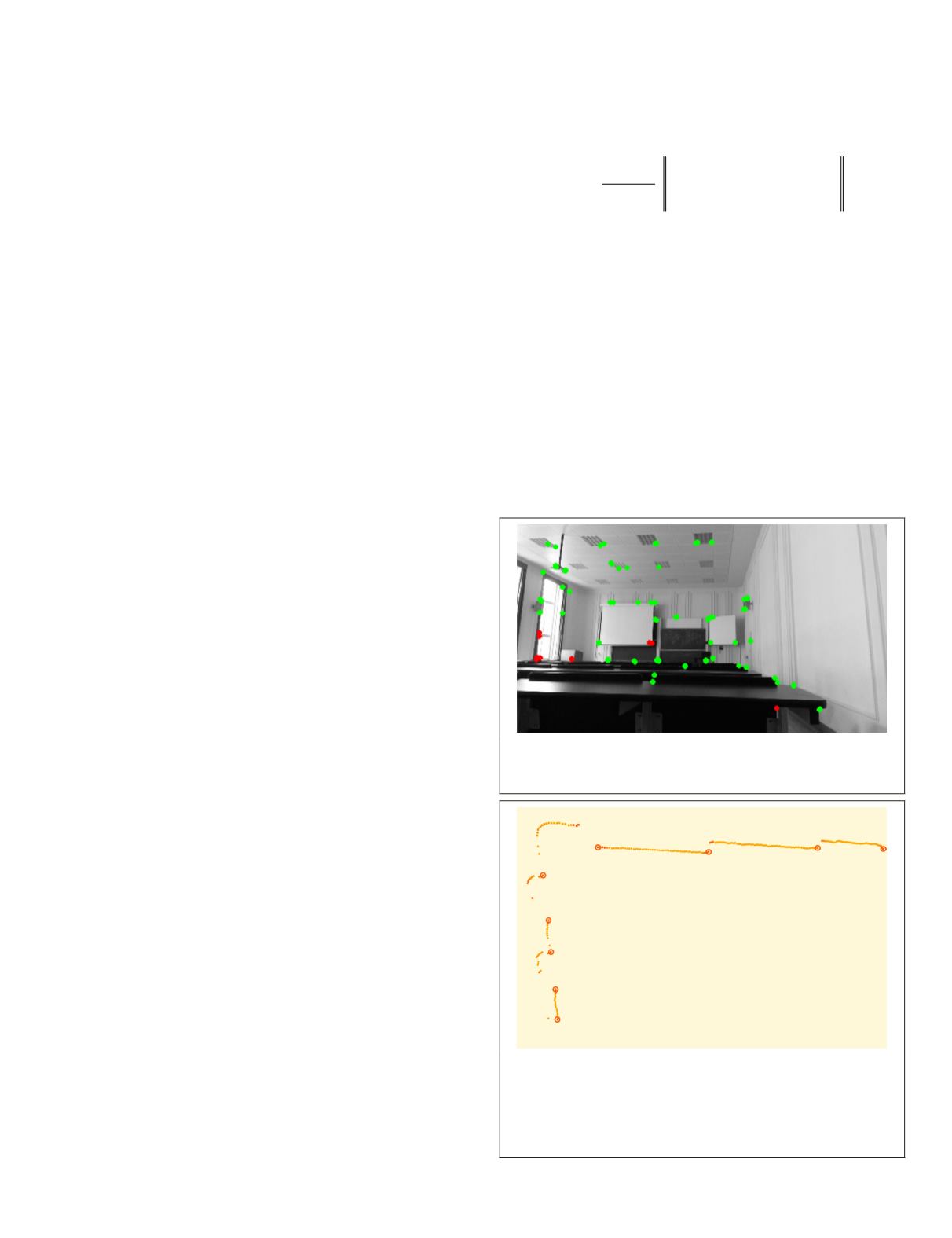
We use
ORB
(Oriented FAST and Rotated BRIEF) (Rublee
et al
., 2011) to extract and match the visual features between
consecutive frames. An example of features that were extract-
ed in a lecture room can be seen in Figure 2. Furthermore, we
refrain from triangulating the depth for visual features since
we only need the visual odometry as an initial guess for the
lidar odometry. This reduces the computational cost.
Lidar Odometry
The lidar odometry method (J. Zhang and Singh, 2014) consists
of two algorithms that run separately. The first algorithm
(sweep to sweep refinement) takes the motion estimation calcu-
lated by the visual odometry as an initial guess that is suscep-
tible to drift. We get motion estimates with a frequency of 10
Hz
from our visual odometry algorithm and apply them to project
our scan points do the beginning of the sweep. The remaining
drift that cannot be determined using the visual odometry, is
considered as slow motion during a sweep;where a sweep is
the rotation from −90° to + 90° or in the inverse direction with
the horizontal orientation as 0°; and thus, can be modeled with
constant velocity. Now, the aim is to determine this drift and
use it to correct distortion in the point clouds that arises due to
the motion of the laser scanner during a sweep.
To extract scan features, the curvature of every 2D scan
point with respect to its neighbors is calculated as:
c i
N
i j
N
i
i j
i
i j
( )
=
⋅ ⋅
⋅
−
(
)
+ −
(
)
=
−
+
∑
1
2
1
X
X X X X
where
X
i
are the 2D-coordinates of a scan point
i
,
N
is the
number of 2D scan points that are considered for the curva-
ture calculation to both sides of
i
in the ordered 2D scan and
|
X
i
|
is the euclidean norm for
X
i
. Because of the scanner’s
resolution, two successive scan points are 0.25° apart. For
our experiments we set
N
= 5, which showed to be robust
amongst different datasets.
The 2D scan points are distributed into four subregions
and sorted based on the curvature values. From every subre-
gion the two points with the largest curvature that also exceed
a threshold are chosen as edge points and the four points with
the smallest curvature that also do not exceed a threshold are
chosen as planar points. We chose a threshold of 0.8 for edge
points and 0.45 for planar points, which showed to be robust
amongst all datasets as well. An example for the feature ex-
traction can be seen in Figure 3.
Figure 2. Image of a lecture room with
ORB
features marked
as dots. Features whose depth was found are marked in green
while red dots correspond to features with unknown depth.
Figure 3. An example of 2D laser scan points for which the
curvature is calculated. Dark orange points correspond to
scan points with large curvature values while light orange
points indicate a small curvature value. Circled points are
extracted as edge points. Since too many planar points were
extracted they are not depicted in this figure.
PHOTOGRAMMETRIC ENGINEERING & REMOTE SENSING
June 2018
359


