Datasets
For our experiments we acquired four datasets of different
characteristics. Before we introduce and discuss the results
that our motion-based approach yields, we want to present
those datasets to give the reader an impression. To create a
representation of the datasets, we used the previously dis-
cussed
SLAM
approach that is presented by J. Zhang and Singh
(2015). Note that no georeferencing was used and we carried
the sensor setup along for all data recordings.
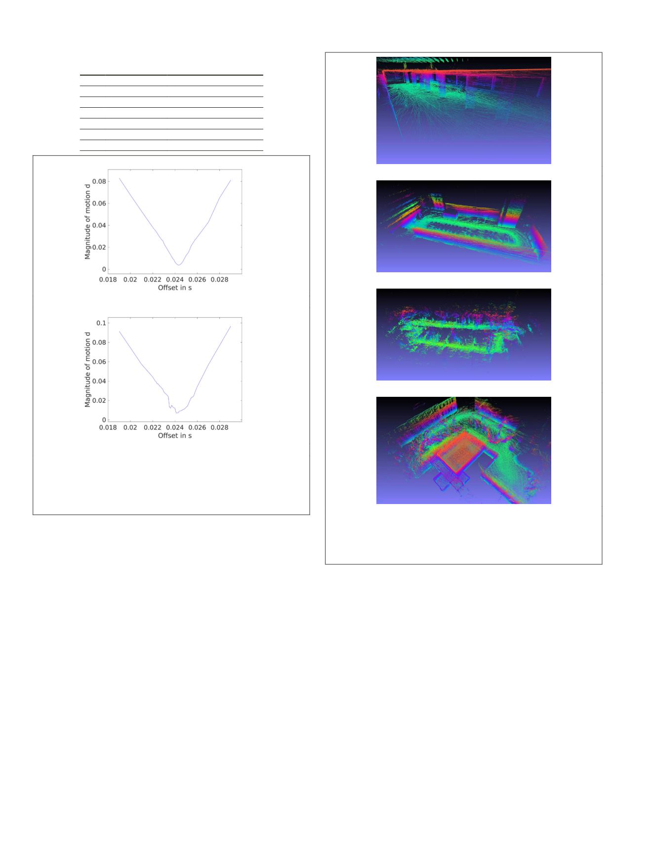
The first dataset contains data that was recorded in an
abandoned metro station. In a period of roughly 159 s we
cover a distance of around 117 m with a maximum velocity of
1.3 m/s and a maximum angular rate of 0.44 rad/s. Moreover,
we finish the measurement in the same spot that we started it
in. The final map can be seen in Figure 6a.
For the second dataset we moved across a parking area. In
a period of roughly 208 s we cover a distance of around 155 m
with a maximum velocity of 1.5 m/s and a maximum angular
rate of 0.61 rad/s. Again, we finish in the same spot that we
started in. In Figure 6b the corresponding map can be seen.
The third dataset was recorded on a cemetery. In a period
of roughly 287 s we cover a distance of around 236 m with
a maximum velocity of 1.4 m/s and a maximum angular rate
of 0.74 rad/s. Once more, we finish in the same spot that we
started in. The final map can be seen in Figure 6c.
For the fourth dataset we choose an environment of several
different characteristics. We started our measurement in
an empty lecture room and finished it in an outside area in
which trees and building facades were present. In a period
of roughly 274 s we cover a distance of around 184 m with a
maximum velocity of 1.9 m/s and a maximum angular rate of
0.91 rad/s. This time we do not finish in the same spot that
we started in. Figure 6d depicts the final map for this dataset.
Motion-Based Approach After Data Acquisition
As explained in the previous section, our motion-based
approach allows us to estimate both the timestamp offset
between laser scanner and motor, and the timestamp offset be-
tween laser scanner and camera. To exclude the possibility of
an unknown correlation between both timestamp offsets, we
evaluated our criteria for different combinations of these two
parameters and came to the conclusion that these parameters
are indeed uncorrelated.
Table 1. Results of the stationary offset computation prior to
data acquisition.
No.
Offset [ms] Magnitude of motion d
1
24.3
0.0037
2
23.4
0.0314
3
23.9
0.0203
4
24.1
0.0070
5
23.8
0.0220
6
24.6
0.0194
(a)
(b)
Figure 5. Results generated by the stationary approach to
calculate timestamp offsets prior to data acquisition. The
measurement graphs belong to experiments whose results
are depicted in Table 1: (a) Experiment No. 1, and (b)
Experiment No. 4.
(a)
(b)
(c)
(d)
Figure 6. Maps generated using the discussed
SLAM
approach. Point clouds are color coded by elevation to
generate 3D perception: (a) Metro station, (b) Parking area,
(c) Cemetery, and (d) Lecture room
362
June 2018
PHOTOGRAMMETRIC ENGINEERING & REMOTE SENSING


