the purpose of avoiding confusion, this paper marks the scale
parameter of this method as
SP
’.
Workflow of Exploring the Relationship Between
Segmentation and Classification
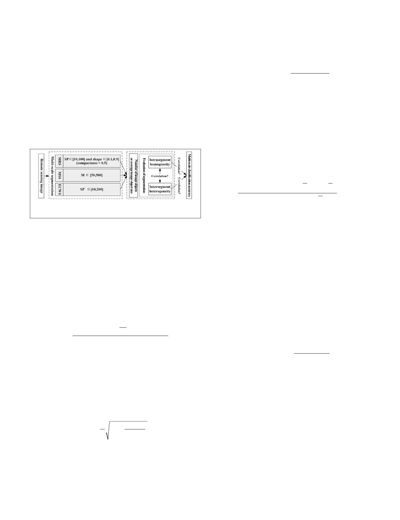
For this study, three scale parameters,
SP
for
MRS
, M for
MS
,
and
SP
’
for
ECW
, are tested. Considering the practical mean-
ings of these three parameters previously discussed, the
influence of scale parameter on image segmentation and
classification are mainly explored. Actually, with the change
of segmentation scale parameter, the segmented image object
amount or the average image object size will correspondingly
change, which results in the variation of intrasegment homo-
geneity and intersegment heterogeneity. Thus, the workflow
of this research is designed as shown in Figure 1, in which
the initial value and the stop value of the scale parameter are
set according to the prior experience.
Figure 1. Frame of exploring the relationship among
homogeneity, heterogeneity and classification accuracy.
Evaluation of Image Segmentation
Generally, there are three types of evaluation methods, and
they are visual evaluation, quantitative evaluation, and indi-
rect evaluation (or application based evaluation) (Li and Xiao,
2007). Based on (Espindola
et al
(2006), this paper uses the
measures based on homogeneity and heterogeneity (Espindola
et al
.,2006; Kim
et al
., 2008; Johnson and Xie, 2011) to quanti-
tatively analyze the scale effect of homogeneity, heterogeneity
with the change of the segmentation parameters.
Intrasegment Homogeneity
Intrasegment homogeneity can be calculated by variance
(
V
i
) of the segmented parcel
i
,
V
f x y
A
f x y
A
i
i
x y R
x y R
i
i
i
=
−
∈
∈
∑
∑
[ ( , )
( , )]
( , )
( , )
1
2
(1)
where
V
i
represents the intrasegment variance of the seg-
mented parcel
i
, and
i
is identifier number of the parcel; A
i
represents the area of parcel
i
;
f(x, y)
is the grayscale value
of pixel
(x, y)
; and R
i
represents the spatial extent of parcel
i
. To describe the degree of homogeneity of the whole seg-
mentation result, the area of the segmentation parcel is used
as the weight to be incorporated into calculating the average
variance of the segmentation result (
AV
)
.
Equation 2 gives the
computation of
AV
:
AV
n
V A
A
i
i
i
i
n
i
n
=
×
=
=
∑∑
1
1
1
(
)
(2)
where
n
is the total number of the segmentation parcels. In
substance,
V
i
represents the variance of the segmentation
parcel, and
AV
describes the heterogeneity within the parcel.
Thus, the lower the value of
AV
is, the higher the homogene-
ity of the segmentation result. To maintain the consistency of
AV
and intrasegment homogeneity, within a serier of seg-
mentation parameter, we used
N
(
AV
)
j
, normalization of
AV
j
,
to represent intrasegment homogeneity at scale
j
. Equation 3
gives the computation of
N
(
AV
)
j
.
N AV
( )
j
= −
−
−
1
AV AV
AV AV
j
min
max
min
.
(3)
Then, at scale
j
, intrasegment homogeneity
N
(
AV
)
j
is
between 0~1. The higher the value of
N
(
AV
)
j
is, the higher the
intrasegment homogeneity at scale
j
is.
Intersegment Heterogeneity
Intersegment heterogeneity can be described by a spatial au-
tocorrelation index that quantitatively represents the spatial
dependence degree between spatial objects. This paper uti-
lizes the Moran Index value to evaluate heterogeneity within
the whole segmentation image (marked with
MI
). The Moran
index is a measure of the spatial autocorrelation, which is
characterized by a correlation in a signal among nearby loca-
tions in space. The formula of computing
MI
is as follows:
MI
n
w y Y y Y
w
y Y
ij
i
j
j
n
i
n
ij
i
i
n
j
n
=
×
× − × −
×
−
=
=
=
=
∑∑
∑
(
(
) (
))
(
) (
(
) )
1
1
1
2
1
∑∑
=
≠
i
n
1
(i j) (4)
w f i j
i j
=
=
( , )
1, if parcel i and parcel j are adjacent
0, if parcel i and parcel j are not adjacent
(5)
where
y
i
and
y
j
respectively represent the average grayscale
value of parcels
i
and
j
;
Y
–
represent the average grayscale
value of the whole original image;
n
is the total number of
the segmentation parcels; and
w
ij
is a constant that denotes
whether parcel
i
and parcel
j
are adjacent (
i
≠
j
;
w
ii
=0
).
In a similar way, the essence of
MI
is the spatial correlation
between the segmentation parcels within the whole original
image and not the direct index to express the intersegment
heterogeneity. In theory, the lower the spatial correlation (the
value of
MI
), the higher the intersegment heterogeneity.
To maintain the consistency of
MI
and intersegment
heterogeneity, within a serier of segmentation parameter, we
used
N
(
MI
)
j
, normalization of (
MI
)
j
, to represent intersegment
heterogeneity at scale
j
. Equation 6 gives the computation of
N
(
MI
)
j
.
N MI
MI MI
MI
MI
j
j
( )
= −
−
−
1
min
max
min
.
(6)
Then, at scale
j
, intersegment heterogeneity
N
(
MI
)
j
is be-
tween 0~1. The higher the value of
N
(
MI
)
j
is, the higher the
intersegment heterogeneity at scale
j
is.
Experiments
Experimental Data
This study used five pieces of image (A, B, C, D, and E) as
shown in Figure 2 (a) ~ (e) in the experiments. Image A is a
multispectral subset aerial multi-band image obtained from
the Erdas Imagine example dataset (the spatial resolution is
unknown). Image B is a subset Ikonos image with 1-meter res-
olution panchromatic band and 4-meter resolution multispec-
tral band (blue, green, red and near infrared). Image C is a sub-
set Quickbird image with 2.4-meter resolution multispectral
band (blue, green, red, and near infrared). Image D is a subset
WorldView-2 multispectral image with 2-meter resolution
PHOTOGRAMMETRIC ENGINEERING & REMOTE SENSING
November 2018
683


