and fragmented of the landscape structure is, the more dra-
matic the fluctuation of the heterogeneity changes, that is why
there are two fluctuations on the intersegment heterogeneity
curves of image D as shown in Figure 4(e) and 4(h). Addi-
tionally, as shown in Figure 4(e) and 4(h), the intersegment
heterogeneity changing tendencies of image D is different,
that is because the scale meanings of the two segmentation
are different. As shown in Figure 6(d) and 6(e), the segmented
image object amount with
MSS
is within [280, 2522], however
the amount with
ECWS
is within (4027, 14737), so the two
curves cannot be absolutely compared by the normalized
N
(
AV
) or
N
(
MI
) values.
However, though the tendency of intrasegment homogene-
ity is not uniform, the overall tendency is upward or with
decrease of image object amount except Image E by using
ECWS
(Figure 5(e)). Figure 4 and Figure 5 also shows that high
intrasegment homogeneity cannot ensure high
OA
because
high intrasegment homogeneity is often companied by under-
segmentation, which will ultimately leads to misclassification.
Scale Effect with Change of Shape Heterogeneity for MRS
This subsection is only for
MRS
. When fixing the
SP
and
changing the shape value, Figure 6(a)~(c) show that the
number of segmented image object decreases with increase
of shape. A high shape parameter value means automati-
cally a low value of the color parameter (or a low weight of
spectral heterogeneity). The neglecting of the importance of
the spectral information in the multispectral images during
the segmentation process has an effect on the result. Figure
4(a)~(c) show that with increase of shape value, the overall
change trends of both intrasegment homogeneity and interseg-
ment heterogeneity are downward, as well as the tendencies
of
OA
as shown in Figure 5(a)~(c). Therefore, it is suggested
to not set shape value too large(the default shape parameter
value in eCognition is 0.1).
Additionally, Figure 5(a)~(c) shows that the classification
accuracy with shape < 0.5 doesn’t obviously differ from each
other when
SP
value is set within a moderate range of 10~30.
Image A and Image B are both with fine spatial resolution
and the borders of building area or residence area in Image A
and Image B are relatively regular, so a compromised shape
value (around 0.5) is appropriate. However, if the shape value
increases (> 0.6), as shown in Figure 3 (for example, shape =
0.9 and
SP
=50), the image objects will become bigger and the
image object number will be less; the borders of the segment-
ed image objects will deviate from the actual border of the
geo-object, which means that under-segmentation exists, so
the intrasegment homogeneity dramatically decreases. For Image
C with spatial resolution of 2.5 meters, the geo-objects in the
study area are fragmented and are mostly of small sizes. In
this situation, the shape feature is not leading factor to seg-
mentation, so Figure 5(c) shows that the changing tendency of
OA
for Image-C does not decrease dramatically as Image-A or
Image-B with decreasing of shape value.
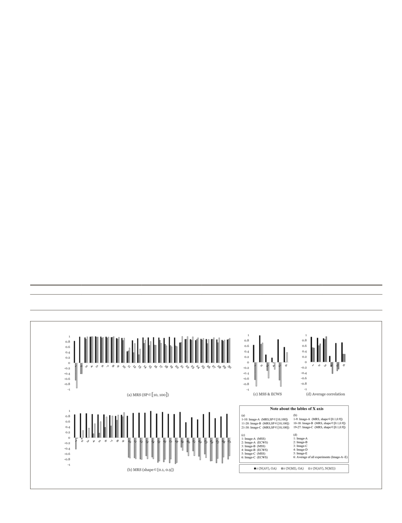
Correlation Analysis of N(
AV
), N(
MI
) and OA
In statistics, the correlation coefficient (r) is a statistic repre-
senting how two random variables co-vary. It can vary from -1
(perfect negative correlation) through 0 (no correlation) to +1
(perfect positive correlation). The corresponding relationship
between correlation coefficient and degree of correlation is
listed in Table 2.
Random variables often represent what is actually ob-
served in an experiment, so the intrasegment homogeneity,
intersegment heterogeneity, and overall classification accuracy
(
OA
) in this research can be regarded as three random variables.
To quantitatively analyze the coupling relationship between
multi-scale image segmentation and classification accuracy
in
GeOBIA
, the correlation coefficient r among the above three
random variables for series of segmentation and classification
are calculated and demonstrated in Figure 7.
Table 2. Relationship between correlation coefficient and degree of correlation.
Degree of correlation
0.00
0.00...±0.30
±0.30...±0.50
±0.50…±0.80
±0.80…±1.00
r
No correlation
Slightly positive/
negative correlation
Positive/negative
correlation
Significantly positive/
negative correlation
Highly positive/
negative correlation
Figure 7. Correlation coefficient of the three random variables (
N
(
AV
),
N
(
MI
),
OA
)
PHOTOGRAMMETRIC ENGINEERING & REMOTE SENSING
November 2018
689


