Correlation Analysis of N(AV) and
OA
From Figure 4~Figure.6, it can be concluded that the overall
classification accuracy is strongly and positively correlated
with intrasegment homogeneity. When spectral heterogene-
ity is low or image object size is small, even though over-
segmentation may happens and intersegment heterogeneity
is low, the high intrasegment homogeneity can ensure the
classification accuracy under the condition that the clas-
sification samples covers all kinds of sub-category. However
when spectral heterogeneity is too high or image object size
is big, low intrasegment homogeneity will inevitably lead
to poor classification accuracy. Figure 7 shows that r(
N
(
AV
),
OA
) is highly positive when changing hetergeneity or shape
parameter From the point of the calculation of intrasegment
homogeneity, the calculation is based on the variance calcula-
tion within the segmented image object as Equation 1, so the
resulted intrasegment homogeneity is reasonable and mean-
ingful to reflect the segmentation scale effect.
Correlation Analysis of N(
MI
) and
OA
Figure 7(a)~7(c)shows 73 groups of correlation analysis
result. 39 out of 73 represents positive correlation and even
significantly positive correlation. As shown in Figure 7(d),
the average r(
N
(
MI
),
OA
) of all 73 groups data is 0.297, which
is positive correlative. However, Figure 7(a)~7(c) also shows
that there is no absolute correlation between
N
(
MI
) and
OA
when changing spectral heterogeneity or shape heterogeneity
because 39 groups indicate the positive correlation and 34
groups indicates negative correlation,, which really conflicts
with the essence of intersegment heterogeneity. There are two
points needed further discussed.
First, when the landscape structure is complex or frag-
mented, there are periorodic waves on landscape heterogene-
ity caused by different hierarchy of natural landscape (multi-
scale landscape). If we truncate the scale sequence, almost
all groups of correlation analysis results represent positive
correlation within a small fluctuation cycle. Additionally, our
classification samples are based on the fine scale and without
considering the hierarchical landscape structure, which may
result in the conflict between change tendencies of interseg-
ment heterogeneity and
OA
.
Second, due to the conflict between theoretical principle
and practical calculation result, the intersegment heterogeneity
calculation as Equation 4 originally proposed by Espindola
et
al
.(2006) is specially analyzed. The intersegment heterogeneity
proposed by Espindola
et al
.(2006) is based on Moran Index
and it computes the quantitative relation to the global average
gray value. However, from the separability of image objects
in
GeOBIA
, the intersegment heterogeneity is oriented toward
the local separability or local heterogeneity between adjacent
image objects. From this view, the rationality of computing
intersegment heterogeneity based on Moran Index should be
further discussed because Moran Index cannot directly reflect
the local heterogeneity. Therefore, a more appropriate interseg-
ment heterogeneity computation should be explored.
Concomitant Relationship Between Intrasegment
Homogeneity and Intersegment Heterogeneity
By comparing r (
N
(
AV
),
OA
) with r (
N
(
MI
),
OA
) in Figure 7 and
combining Figure 4, it can be concluded that intrasegment
homogeneity is more important than intersegment heteroge-
neity in
GeOBIA
because the classification accuracy is strongly
and positively correlated with intrasegment homogeneity.
However, the conclusion summarized above does not mean
intersegment heterogeneity is unimportant. Theoretically,
high intersegment heterogeneity means high separability
between classes, so
r(
N
(
MI
),
OA
) should be theoretically posi-
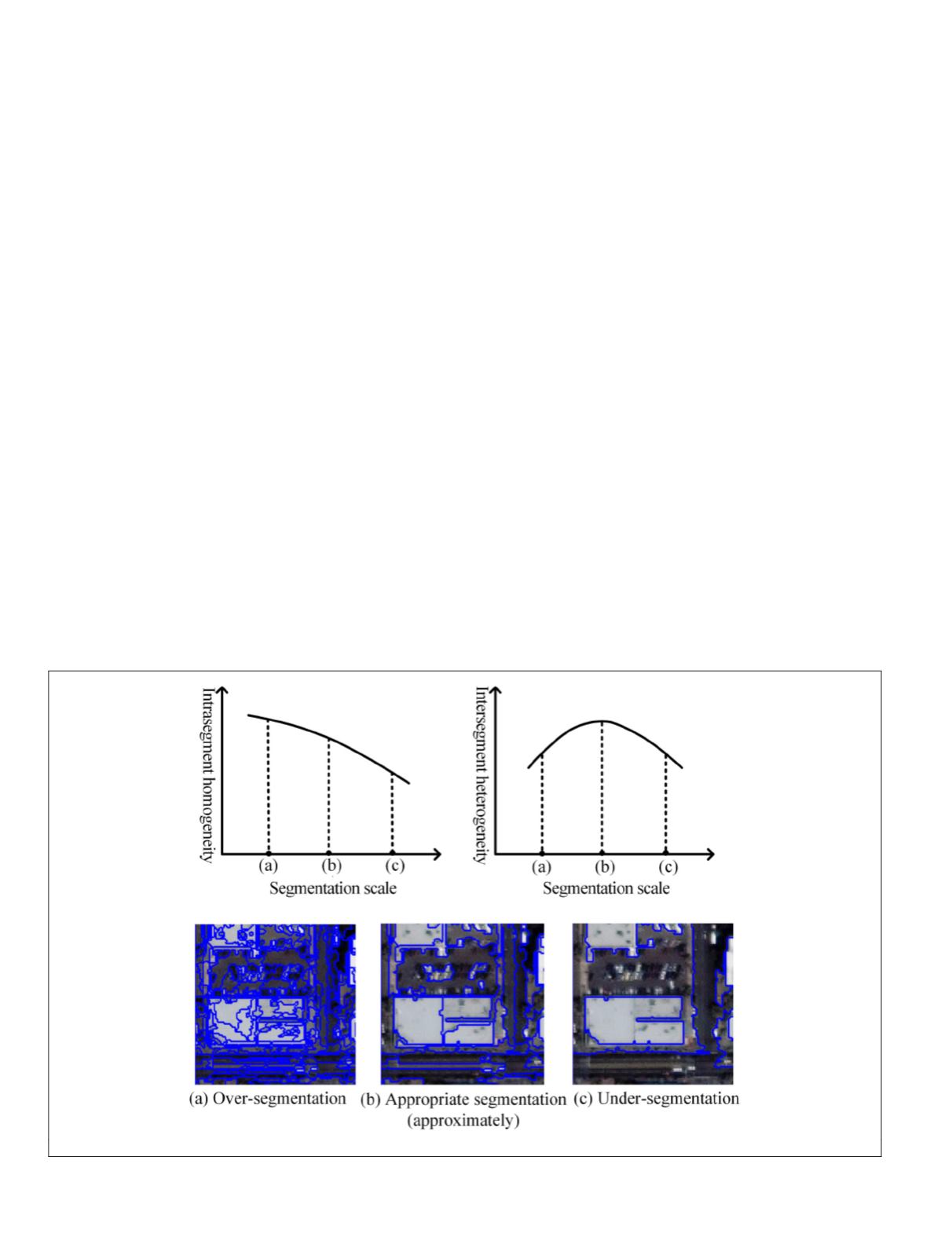
tive; additionally, with increase of segmentation scale or the
segmentation image object size, the intrasegment homogene-
ity decreases and the intersegment heterogeneity theoretically
increases first and then decreases after a certain scale. This
certain scale is theoretically the optimal scale.
To simply reflect this speculation, Figure 8 illustrates the
ideal change trend of intersegment heterogeneity with image
Figure 8. Ideal concomitant relationship between intrasegment homogeneity and intersegment heterogeneity.
690
November 2018
PHOTOGRAMMETRIC ENGINEERING & REMOTE SENSING


