soil background information is minor, and a constant low
NDVI
value was often used to represent the background information
(Lu
et al.
2003; Helman
et al.
2015). Accordingly, we used a
constant value of 0.1 to represent the background contribution
based on another study in our study area (Hill
et al.
2016). The
constant value was subtracted from the type 1 variation. The
detailed procedure of the frequency decomposition consists of
five steps (Figure 4).
Step 1:
Retrieve type 1 variation
. The type 1 variation is re-
trieved from the
NDVI
time series using the statistical method
STL
(Cleveland
et al.
1990). We also considered using the Fou-
rier transform to retrieve type 1 variation and remove noise.
But then we had to determine an arbitrary frequency thresh-
old for noise and long-term variation, which could be contro-
versial for this high temporal resolution dataset. One the other
hand,
STL
is a popular method for decomposing time series,
and outputs trend component and seasonal component. The
trend component is equivalent to the type 1 variation that is
added to the woody variation after the frequency decomposi-
tion. The seasonal component, however, contains both type 2
and 3 variations as defined in this study.
Step 2:
Separate type 2 and 3 variations
. The seasonal com-
ponent from the
STL
is converted to a sequence of frequen-
cies. By comparing the amplitude distribution of frequency
sequence (Figure 3), we assume that frequencies from 1–5
cycles per year have most of the seasonal component in-
formation and enough variation to determine the regres-
sion coefficients. So, we use frequencies from 1–5 cycles to
represent type 2 variation and higher frequencies to represent
type 3 variation. A multi-frequency combination of one cycle
per year (red), two cycles per year (green), and three cycles
per year (blue) is shown in Figure 5. The type 3 variation is
restored after the decomposition at Step 4.
Step 3:
Build frequency decomposition model
. The coeffi-
cients
c
1
and
c
2
of woody and herbaceous components are es-
timated using the type 2 frequencies of mixed pixels based on
Equation 2. Common to both regular linear endmember analy-
sis and frequency decomposition is the likelihood of deriving
negative fractions. In time series analysis, the derived unre-
alistic results show high
NDVI
in dry seasons and low
NDVI
in
rainy seasons. Correspondingly, distinctive phase differences
would occur at the annual frequency between the mixed pixel
and the derived fractions. To avoid the occurrence of unreal-
istic fractions, an annual phase difference threshold between
the original time series and the decomposed time series
was used in this study. If the phase difference surpassed the
threshold, the corresponding coefficient
c
1
or
c
2
was set to
zero. After a systematic test using different time intervals, this
study used a one-month difference as the threshold.
Step 4:
Restore type 3 variation
. The type 3 varia-
tion is assigned back to woody and herbaceous
components based on the amplitudes of
c
1
and
c
2
:
F V c F V
abs c
abs c abs c
F V
s
h
( )
=
( )
+
( )
( )
+
( )
( )
1
1
1
1
2
(3)
where
F
S
(
V
1
) is the seasonal frequencies of the
woody endmember, and
c
1
F
S
(
V
1
) is the derived
seasonal frequencies of woody components.
F
h
(
V
)
he short-term signal from the mixed pixel,
ile
F
(
V
)
is the derived full woody frequency
uence of the mixed pixel. The full herbaceous
uency sequence is assembled in the same
way.
Step 5:
Construct separate time series for herba-
ceous and woody vegetation
. The full woody and
herbaceous frequency sequences are transformed
to
NDVI
time series of herbaceous and woody
components. The type 1 variation is added to the
woody time series. The final outputs are woody
and herbaceous eight-day
NDVI
time series from
2002 to 2011.
Selection of Endmembers
The seasonal frequencies (from step 2) are used
to find pure woody and herbaceous pixels across
the whole study area. Unsupervised classification
is first applied to the seasonal frequencies dataset
using the Iterative Self-Organizing Data Analysis
Technique. The classification divides the dataset
into 100 groups. Pure woody and herbaceous
classes are then determined by comparing pixels
within each class to the Google Earth images. A
total number of 11 390 and 6616 relatively pure
woody and herbaceous pixels, respectively, are
selected. The endmembers were calculated by
averaging woody or herbaceous time series from
multiple pure pixels, which aimed to represent
the general seasonal variation of various species
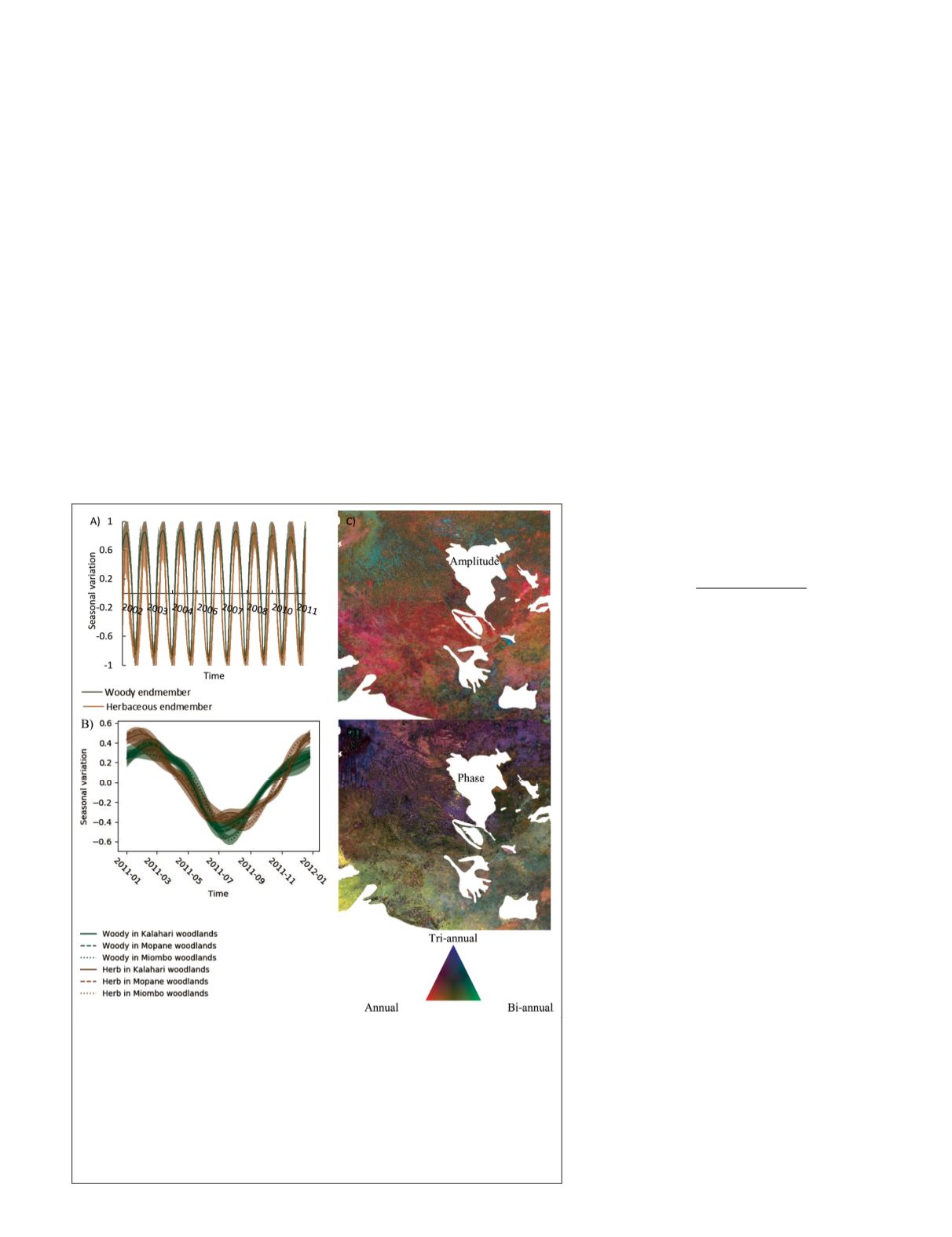
Figure 5. Panel a) shows the time series converted from endmember
seasonal frequencies. The buffer areas surrounding the solid lines show
the standard deviation (
STD
) of pixels within each endmember. Panel
b) shows the end member time series in 2011 for major ecosystems:
Kalahari (Kalahari Acacia-Baikiaea woodlands); Mopane (i.e. Angolan
Mopane, Zambezian and Mopane woodlands); and Miombo (i.e. Angolan
Miombo, central Zambezian Miombo, Southern Miombo woodlands).
The buffer areas indicate the
STD
. Panels c) and d) demonstrates the
spatial distribution of amplitude or phase as composition of once a year
(red), twice a year (green), and three times a year (blue) frequencies.
PHOTOGRAMMETRIC ENGINEERING & REMOTE SENSING
July 2019
513


