HSI Pixel Preprocessing
MH
prediction (Sullivan 1993) has been successfully used in
HSI
reconstruction and classification (C. Chen
et al.
2014). For
HSI
classification,
MH
preprocessing is first applied based on
piecewise-continuous image characteristics and the spectral
similarities between a testing pixel and its neighbors. This
preprocessing leads to the representation of a testing pixel as
a linear combination of its neighboring pixels. In this article,
MH
prediction is used for hyperspectral feature extraction and
image reconstruction, where the reconstructed images show
more distinctive characteristics. Given an input pixel vector
y
∈
R
b
of an
HSI
,
H
= [
h
1
, …,
h
s
]
∈
R
b×s
is a matrix consisting of
the neighboring-pixel vectors of the input pixel
y
, where
b
is
the number of spectral bands,
s
=
n
s
×
n
s
–1 is the number of
neighboring pixels, and
n
s
is the neighborhood size. Then the
reconstruction problem can be formulated as the following
least-squares problem:
=
w H
= =
ˆ argmin
ˆ
ˆ
w
y
y H
w
where
y
ˆ is the reconstructed pixel vector and
w
is an
s
× 1
vector of linear representation coefficients corresponding to
all the columns of
H
. In most cases, a regularization term is
added to Equation 5 to impose a
L
2
penalty on the norm of
w
ˆ ,
as follows:
(
)
= =
=
−
ˆ argmin
ˆ
ˆ
,
w
y Hw w
y Hw H H H
H y
+
+
w
2
2
2
2
γ
γ
Λ
Λ Λ
T
T
T
(6)
where
γ
is a weight parameter and
Λ
is the Tikhonov matrix.
In the case of
MH
prediction, the matrix
Λ
takes the following
diagonal form:
Λ
=
−
−
y h
y h
1 2
2
2
2
0
0
s
.
(7)
The matrix
Λ
performs the reconstruction task as follows. The
hypotheses that are most dissimilar from the original pixel
vector should be given smaller weights, while those with high
similarities are given larger weights (C. Chen
et al.
2014).
After all, the pixels in an
HSI
are reconstructed using Equation
6. The new reconstructed hyperspectral features, which com-
bine spatial and spectral information, can be used as classifier
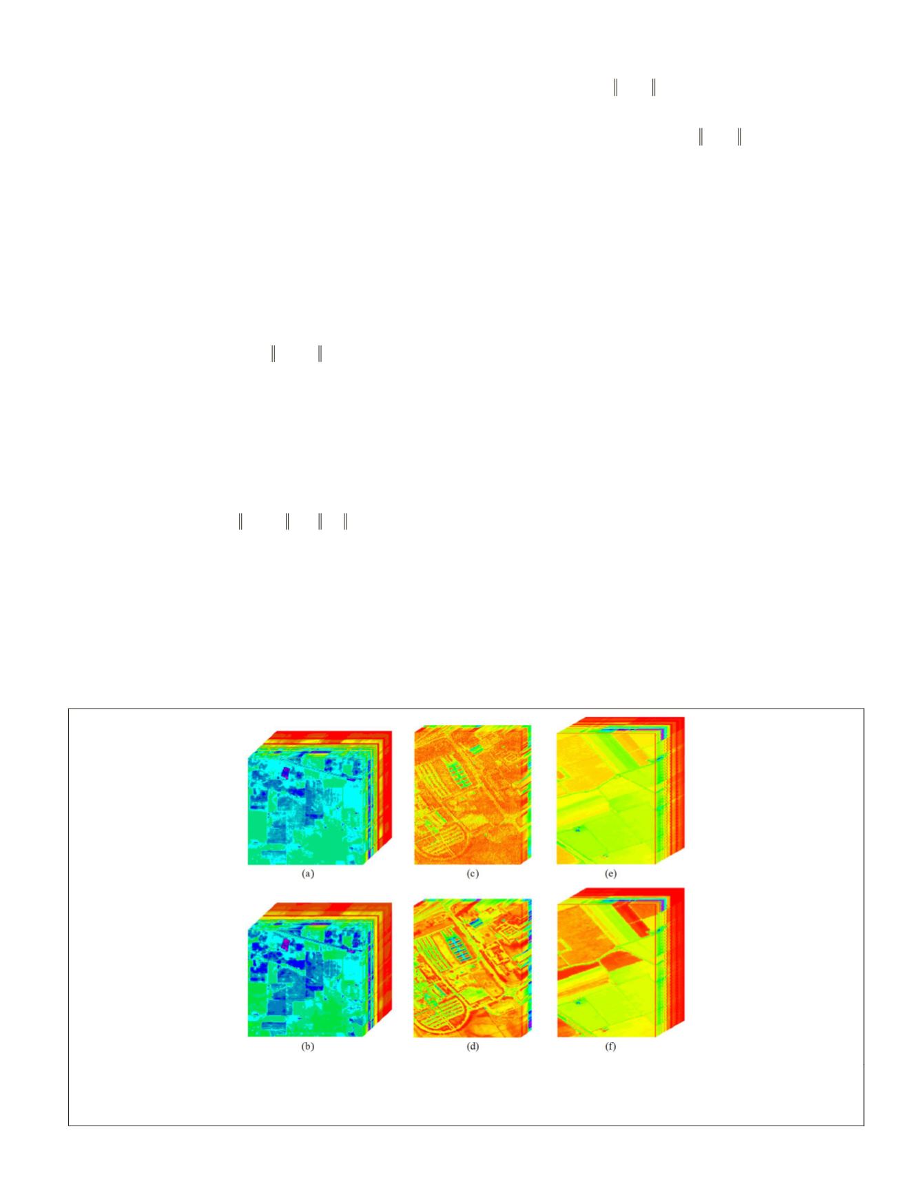
input. The samples of original and preprocessed images are
shown in Figure 4. It can be seen that preprocessing improves
the discrimination of pixels to some extent.
Collaborative Sparse Coding with Smoothness Regularization
ation using
CSCSR
is explained in
f pixels from the
HSI
are randomly
ry for the
CSCSR
scheme, while the
s testing samples. Sparse coding
sparse representations of the testing
pixels with respect to the model dictionary. After that, the
collaborative representation errors for the different classes are
computed and the class of a testing pixel is determined as the
class of the training samples with the minimum representa-
tion error. The proposed
CSCSR
scheme exploits the spatial
relationship between neighboring pixels to improve
HSI
-clas-
sification performance.
The proposed
CSCSR
method is based on sparse coding
combined with
l
1
-norm regularization. For sparse coding, the
training pixels are used to form a dictionary with respect to
which the sparse codes of a testing pixel can then be ob-
tained. Then the testing pixel is assigned a certain class ac-
cording to the representation error. However, an
HSI
may have
hundreds of narrow bands with strong correlation between
pixels. In this case, a direct application of sparse coding
may not achieve satisfactory classification performance even
with
MH
prediction. To deal with this problem, a collabora-
tive sparse-coding (
CSC
) scheme combined with
l
1
-norm
Figure 4. Preprocessing of samples of hyperspectral images: (a) the original Indian Pines image (145×145×200), (b)
the preprocessed Indian Pines image (145×145×200), (c) the original University of Pavia image (610×340×103), (d)
the preprocessed University of Pavia image (610×340×103), (e) the original Salinas image (512×217×204), and (f) the
preprocessed Salinas image (512×217×204).
PHOTOGRAMMETRIC ENGINEERING & REMOTE SENSING
September 2019
661


