Smoothness regularization:
The third term,
λ ω
2
2
2
1
j
j
j
α
α
−
=
∑
k
,
is a smoothness-regularization term, where
ϖ
= [
ω
1
, …,
ω
k
]
∈
R
l×k
is a weight vector,
ω
j
is the weight
parameter assigned to the
j
th pixel
y
j
in a patch, and
α
– = mean (
α
1
, …,
α
k
)
is the mean vector. The aim of the third
term is to reduce the variance of the sparse representation
vectors
α
j
, making them similar to each other. This regulariza-
tion term is based on the fact that neighboring pixels are more
likely to be of the same class due to the spatial regularity and
continuity properties of
HSIs
. Consequently, neighboring pixels
in an image patch most likely have similar sparse representa-
tion vectors. The similarity can be weighted based on two
measures. One measure is the spatial distances between neigh-
boring pixels and the central pixel: if these distances increase,
the similarity between the correspo
tion vectors should decrease. The ot
ity in intensity value between neigh
tral pixel: the more similar the neig
the more similar their correspondin
vectors will be. Then the weight vector
ϖ
is defined based on
the spatial distance and intensity value similarity measures, in
this article, as the Gaussian radial basis function kernel:
2
2
ω
σ
σ
τ
ω
j
j
x
c
x
j
y
c
y
j
c
j
l
l
l
l
= −
−
−
−
−
−
=
exp
,
2
2
2
2
2
2
2
y y
s. t.
0
0 15
0 15
0 80
1
0 80
,
.
,
.
.
,
.
,
ω
ω
ω
ω
j
j
j
j
≤
< <
≥
(10)
where (
l
x
j
,
l
y
j
) is the spatial location of
y
j
, (
l
x
c
,
l
y
c
) is the spatial
location of
y
c
, and
σ
and
τ
are the variances of the Gaussian
function for the spatial distance and intensity value similar-
ity, respectively. Low and high thresholds for
ω
j
are 0.15 and
0.80. One key feature of our method is the identification and
exclusion of neighboring pixels whose classes are different
from that of the central pixel. Such neighboring pixels are dis-
carded because of their small or even negative impact on
HSI
classification. Those pixels with weights smaller than 0.15 are
considered to be highly different from the central pixel and
are hence discarded in the classification. On the other hand,
those pixels with weights larger than 0.80 are considered to
be of the same class as the central pixel and therefore have
the maximum weight in the classification process. The pixels
with weights between 0.15 and 0.80 are partially similar to the
central pixel, and hence their corresponding weights remain
unchanged and contribute proportionally to classification
(H. Zhang
et al.
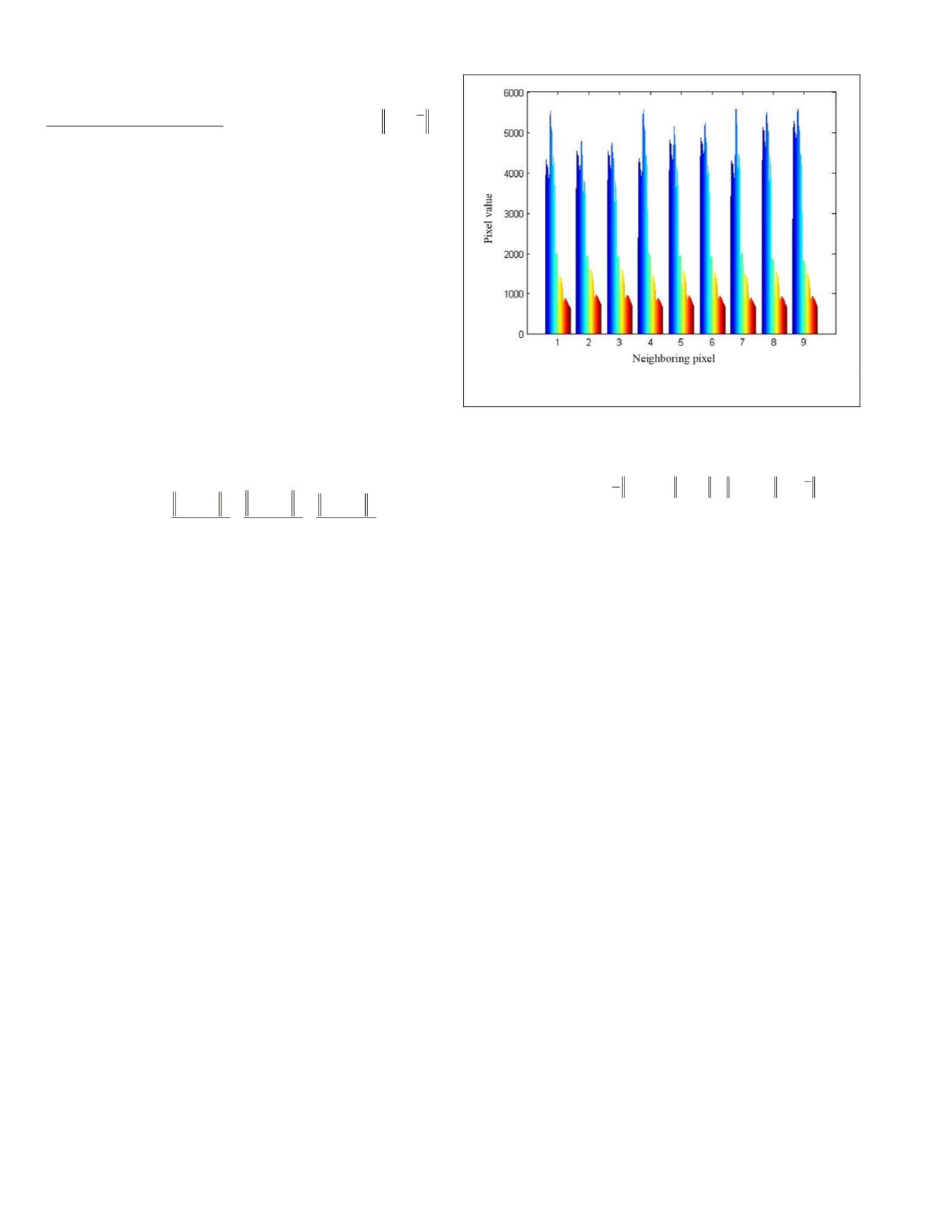
2014). For example, a patch with nine pixels
denoted by [
y
1
,
y
2
,
y
3
,
y
4
,
y
5
,
y
6
,
y
7
,
y
8
,
y
9
] is shown in Figure
9, where
y
5
is the central pixel and the associated weight
vector is
ϖ
= [0.37, 1, 1, 0.64, 1, 1, 0.40, 1, 0.85] . The weights
indicate that the pixels
y
2
,
y
3
,
y
6
, and
y
8
are the most similar to
y
5
and hence contribute the most to the classification decision.
Optimization Algorithm
For the
CSCSR
method, the objective function in Equation 9
is minimized to determine the class of each testing pixel in
HSIs
. Since the parameters
λ
1
and
λ
2
are constants, the weight
vector
ϖ
is computed from Equation 10, and the dictionary
D
is obtained in advance from class samples, it only needs to
solve for the optimal
SC
matrix
Ψ
ˆ = [ˆ
α
1
, …, ˆ
α
k
]. As the sparse
coefficient vectors of different pixels are independent, these
vectors can be optimized independently. Specifically, for an
image patch
Y
= [
y
1
, …,
y
k
], the corresponding optimization
problem is
+
+
λ
λ
y D
ˆ , , ˆ
min
, , ,
α
α
α
α
α
α
α α
α
1
2
2
1
1
2
2
2
1 2
1
2
…
…
k
k
=
−
−
j
j
j
j
j
ω
=
∑
j
1
k
.
(11)
For the optimization problem in Equation 11, the first and
the third terms in the objective function are convex qua-
dratic functions of
α
j
. However, the second term is a Lasso
regularization term that makes the objective function not
continuously differentiable (Lee
et al.
2007). Hence, the most
straightforward gradient-based methods are difficult to apply.
In this article, the feature-sign search algorithm (Lee
et al.
2007) is exploited and improved with smoothness regulariza-
tion to solve the optimization problem in Equation 11. The
algorithmic details are summarized in Algorithm 1. Two key
points in this algorithm are the iterative differentiation of the
smoothness-regularization term and the update of the mean
of the sparse representation vectors. Usually, the last iterative
estimate of this mean is substituted into the next iteration.
However, this approach does not work for the feature-sign
search algorithm, and thus an alternative approach is needed
for our
CSCSR
scheme. From earlier, the representation
y
=
D
α
+
ε
is based on the sparse-signal theory. Here, it is assumed
that a testing pixel can be perfectly reconstructed by the
dictionary—that is,
y
=
D
α
. The sparse coefficient vector as-
sociated with a pixel can then be computed as
α
j
=
D
–1
y
j
, and
hence the mean vector is
α
– = mean(
α
1
, …,
α
k
) =
D
–1
·
y
– , where
y
– = mean(
y
1
, …,
y
k
). The satisfactory classification results
demonstrate the validity of this assumption.
After obtaining the
SC
vectors of all testing pixels in an
HSI
, the
HSI
is reconstructed through the equation ˆ
y
≈
D
α
, as
shown in Figure 10. From the output images, it can be said
that the
SC
,
CSC
, and proposed
CSCSR
methods can faithfully
represent the input image. More importantly, the reconstruct-
ed images based on our proposed
CSCSR
method look more
continuous and clearer. That means that the
CSCSR
method
better represents pixels, reduces the correlation between
them, and leads to better
HSI
classification.
Classification
Once the
SC
vectors are calculated, the class of the central
testing pixel of an input image patch can be determined. The
classification is based on finding the class with the minimum
overall representation error of the image patch. For class
i
,
this error can be computed as
erspectral-image patch with nine
intensity profile for each pixel.
664
September 2019
PHOTOGRAMMETRIC ENGINEERING & REMOTE SENSING


