classes,
D
i
is the subdictionary from class
i
, and each column
in
D
i
is a basis vector for representing
y
. Let
α
denote the
sparse-coding coefficients of
y
with respect to dictionary
D
.
Based on sparse-representation theory,
y
can be represented by
a linear combination of the atoms of dictionary
D
as
y
=
D
α
+
ε
(1)
where
ε
is the representation error. This sparse representation
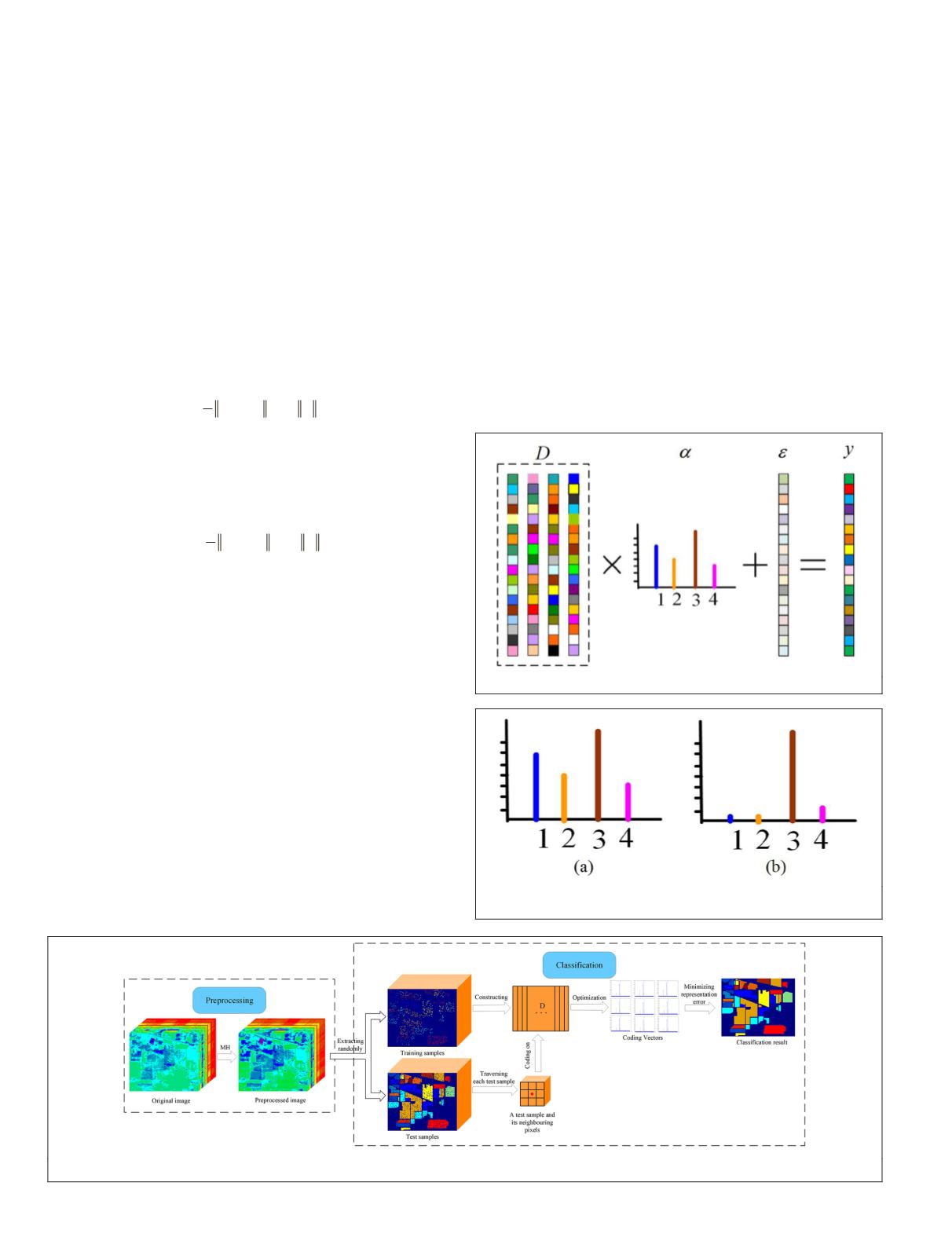
can be visualized as shown in Figure 1.
Ideally, a testing sample should be mainly represented
by dictionary atoms of the same class. In other words, the
representation coefficients associated with all subdictionaries
should be zero except for those associated with the subdic-
tionary of the true class of the testing sample. Therefore,
α
should be a sparse vector. The sparsity of
α
can be measured
by its
l
0
-norm, which counts the number of nonzero entries in
α
. The nonzero entries of
α
correspond to the weights of the
selected dictionary atoms,
min
α
α
1
2
2
2
y D
−
where
λ
is a regularization parameter. Since the solution of the
minimization problem in Equation 2 is NP-hard, the
l
0
-norm
can be replaced by an
l
1
-norm approximation, which leads to
the relaxed sparse-coding problem (L. Zhang
et al.
2011),
y D
− +
min
α
α
α
1
2
2
2
1
λ
(3)
Sparse signal modeling generally leads to better classifica-
tion outcomes. As shown in Figure 2, sparse coding leads
more easily to the conclusion that the testing sample should
belong to Class 3. Sparse signal classification can be based on
the representation error. Actually, each subdictionary consists
of several atoms, not just one. All atoms in the subdictionary
with the same class as the testing sample should then have
large representation coefficients. As a result, the representa-
tion error of the true class of the testing sample should be the
minimum. This minimum-error criterion can be used to clas-
sify testing samples,
label (
y
) = arg min
i
{
e
i
},
(4)
where
e
i
=|
y
–
D
i
α
ˆ
i
|
2
and
α
ˆ
i
| is the sparse representation as-
sociated with class
i
.
Proposed Method
Our
HSI
-classification scheme has two major stages. The first
stage is the extraction of discriminative spectral and spatial
features. However,
HSI
feature extraction is challenging due to
the typically high number of spectral bands. In our work,
HSI
data are preprocessed with
MH
prediction, and the resulting
patterns used as features. In fact, spatial and spectral features
can be merged to boost
HSI
-classification performance. In the
second stage, pixels are classified based on their spatial and
spectral features. Based on spatial continuity of
HSI
data, a
collaborative filtering approach is adopted to improve classi-
fication performance. Specifically, the output class of a testing
pixel is determined not only by its own features but also by
those of its neighboring pixels. The contributions of those pix-
els can be weighted by their similarities to the central pixel.
More specifically, the workflow of our scheme is as follows.
First, training samples are selected to construct a dictionary
from each class while the remaining samples are used for test-
ing. Next, for each testing pixel, small image patches (e.g., 3
× 3) are used to compute sparse-representation vectors based
on sparsity and smoothness-regularization terms. Finally, the
pixel is decided to be the class with
sentation error. A flowchart of the
in Figure 3.
Figure 1. Dictionary-based signal representation.
Figure 2. The coding vector: (a) the original coding without
sparsity, and (b) the sparse coding.
Figure 3. A flowchart of the proposed method of hyperspectral-image classification.
660
September 2019
PHOTOGRAMMETRIC ENGINEERING & REMOTE SENSING


