labeled data (see Table
3). In the Pavia Univer-
sity data set, we ran-
domly divided the total
available data into two
parts: 75% for training
and 25% for testing
(see Table 4). Then, for
the 75% training data,
we randomly selected
thirty samples in each
class as the initial
labeled data.
In the experiments,
for every algorithm, ten
runs were executed on
each image with differ-
ent initial labeled data. The experimental simulation environ-
ment is Inter
®
Core™ i7-6700HQCPU@2.6Ghznotebook, and
its memory is 16 G, and the operating system is Windows 10.
Using the Python Scikit-learning algorithm package to simulate
the experiment. The adopted classifier is
SVM
based on the
radial-basis-function kernel. There two parameters for the
SVM
classifier, i.e., the Gaussian kernel parameter G and the regu-
larization parameter C. They are tuned via grid search and the
searching space defined by G={2
-15
,2
-13
,……,2
3
} and C={2
-5
,2
-3
,…
…,2
15
} (Chang and Lin 2011; Mountrakis, Im, and Ogole 2011).
Moreover,
DSC-CASSL
has two parameters Q and m, where m
is the size of the candidate query set and Q is the size of the
actual query set. We set
Q
= 10 and
m
= 40. At each iteration,
10 samples were selected for manual labeling. The principle
of active learning is to use fewer labeled samples to get the
better training effect. Therefore, the number of labeled samples
represents the labor cost and measures the consumption of
active learning in the iterative phase. Because of the technique
of batch extraction, the minimum unit cost of manual labeling
is Q, and it is the number of batch samples. The cost of manual
labeling as follows:
Cost
= +
(
)
× − = + ⋅
( )
< < +
(
)
N h h Nh h P N p P N
1
1
2
1
2
1
,
(9)
where P(N) is the model precision, the v
specified as Overall Accuracy (OA), AA,
For example, if require OA = 80%, the cost of active learning
can be calculated, setting
Q
= 10 and
p
= 80%, and if
N
= 15
just match Equation 10, the Cost as follows:
Cost
= × + × =
15 10
1
2
10 155
(10)
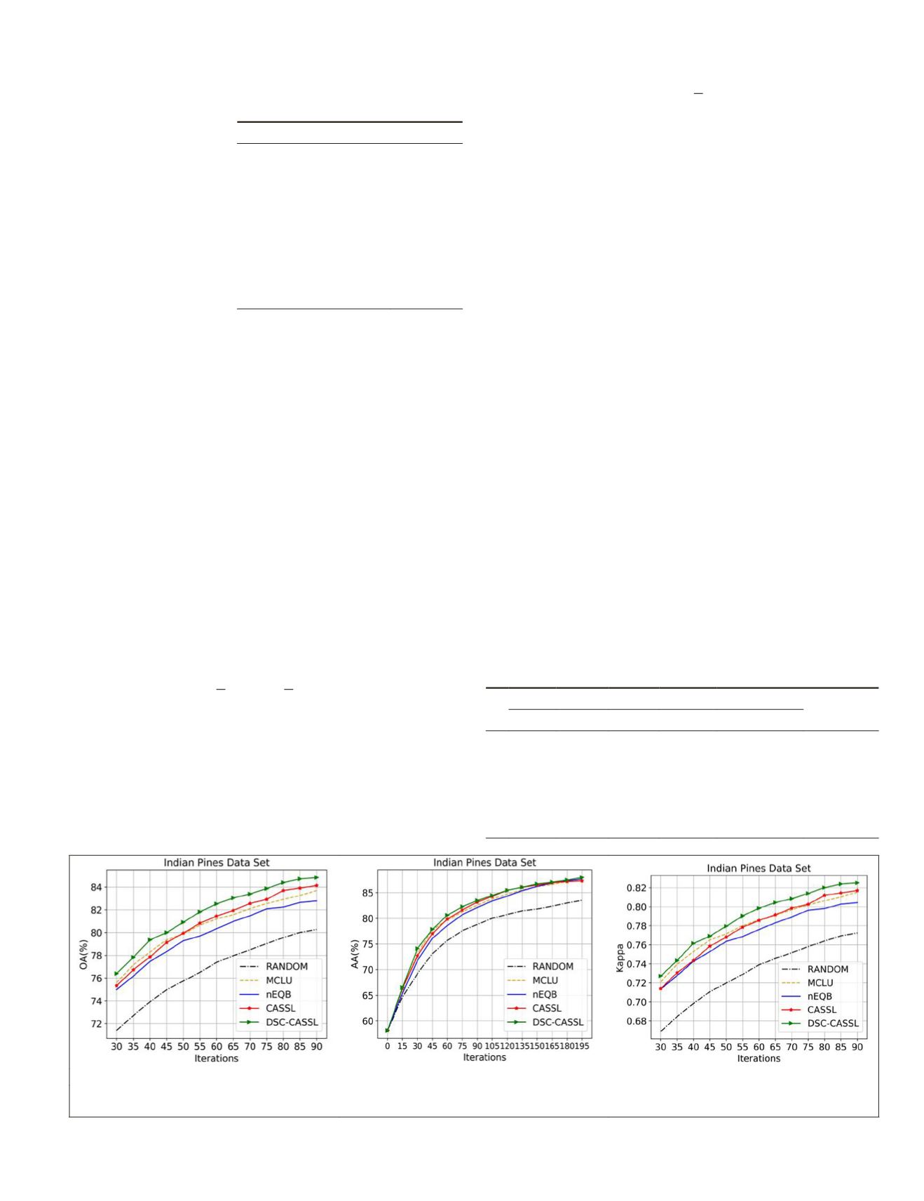
Experiment on the Indian Pines Data Set
To demonstrate the effectiveness of the proposed framework,
we compare the
DSC-CASSL
with
CASSL
,
MCLU
,
nEQB
, and Ran-
dom Sampling (RS) techniques. Firstly, regarding the single
strategy of active learning such as
MCLU
and
nEQB
, this plot
reveals the advantages of using an
AL
heuristic instead of RS.
We can observe that
MCLU
outperforms than
nEQB
. This can at-
tribute that the
nEQB
technique results in poorer classification
accuracies with small values of Q and limited initial labeled
samples. The computational complexity of
nEQB
technique is
very high in the case of selecting few samples. The interesting
thing is that
CASSL
works worse than
MCLU
in average accu-
racy (AA) before the labeled data is less than 700. Because the
initialization samples of all compared methods are limited,
it leads to low confidence in the construction of the train-
ing model and bias in the preestimation of the pseudolabels.
When the training samples reach a certain amount, the ac-
curacy of the pseudolabels is guaranteed and
CASSL
starts to
outperform the
MCLU
.
Taking into account the Indian Pines data set, before the
newly labeled data reaches 150,
DSC-CASSL
doesn’t perform
better than other comparison methods. The main reason is
that the double-strategy-check framework may have a “cold
start” problem. It is widely acknowledged that if the size
of initial labeled data set is too small, the performance of
pseudolabeling procedure could be much deteriorated, which
is known as the “cold start” problem. If the initial training
set does not match the class distributions, it is impossible to
obtain an effective classifier at the very initial stage. When the
algorithm runs over the 15 times, we can observe that
DSC-
CASSL
consistently outperforms other methods. Table 5 shows
five comparative algorithms in different iterations. In Figure
Table 4. Numbers of samples for
the corresponding classes of the
Pavia University data set.
Class Name
No. Samples
Asphalt
6631
Gravel
2099
Metal sheet
1345
Bitumen
1330
Shadows
947
Meadows
18 649
Trees
3064
Bare soil
5029
Self-blocking bricks
3682
Table 5. The comparison of Overall Accuracy between the com-
pared algorithms and
DSC-CASSL
on the Indian Pines data set.
Algorithm, %
Increase, %
EQB CASSL DSC-CASSL
4.99 75.33
76.40
+1.42
45 74.99 79.37 78.34 79.13
80.00
+1.10
60 77.39 81.20 80.34 81.45
82.53
+1.33
75 79.04 82.55 82.09 82.92
83.87
+1.15
90 80.27 83.69 82.79 84.13
84.83
+0.83
(a)
(b)
(c)
Figure 6.
OA
,
AA
, and Kappa results of the different algorithms on the Indian Pines data set. (a) Scaled-up version
OA
. (b)
AA
.
(c) Scaled-up version Kappa.
PHOTOGRAMMETRIC ENGINEERING & REMOTE SENSING
November 2019
847


