train two verification classifiers. At this time, the two verifica-
tion classifiers have a large difference in sample distribution
due to different strategy choices. Meanwhile, the unlabeled
data with pseudolabels and the unlabeled data are predicted
by base model. We denote the label assigned by base model
as
Label
1
. We use
L
Q
1
to train check classifier 1 and use
L
Q
2
to train check classifier 2. Finally, the unlabeled data with
pseudolabels and the unlabeled data are predicted by check
classifier 1 and check classifier 2, respectively. When the base
classifier and two check classifiers obtain the same results on
an unlabeled sample, this denotes that the result is reliable
and then this unlabeled sample will be assigned a pseudola-
bel. On the contrary, if three classifiers have different classifi-
cation results on an unlabeled sample, this unlabeled sample
will be put back in to the unlabeled set for the next iteration.
As the algorithm continues to iterate, the performance of the
classifiers is improved constantly.
When the performance of base classifier and check classifi-
ers has similar generalization capabilities, it indicates that we
can’t obtain enough valuable representative and discrimina-
tive information. Under the circumstance,
CASSL
immediately
finished the improvement of the classification performance.
Compared with the
CASSL
,
DSC-CASSL
exits the part of semisu-
pervised and enter ESAL for next iteration.
DSC-CASSL
only ter-
minates when it reaches the limit iteration times. This can be
attributed to the fact that three classifiers are always making
the same decision is not the end of the
DSC-CASSL
algorithm,
it just means that the algorithm can’t obtain more valuable
information from unlabeled data. In this case, the framework
finishes the SSL part and enters into ESAL part for further im-
proving the performance. As one part of
DSC-CASSL
framework,
ESAL is utilized as a backup process to enhance the imperfect
end condition. It will provide more searching space to select
the informative unlabeled data. Lastly, the performance of fi-
nal combination is superior to the traditional
CASSL
for remote
sensing scene classification. The flowchart of the
DSC-CASSL
algorithm is illustrated in Figure 1, and the pseudocode of the
DSC-CASSL
algorithm is illustrated in Algorithm 2.
Experiments and Analysis
Data Sets
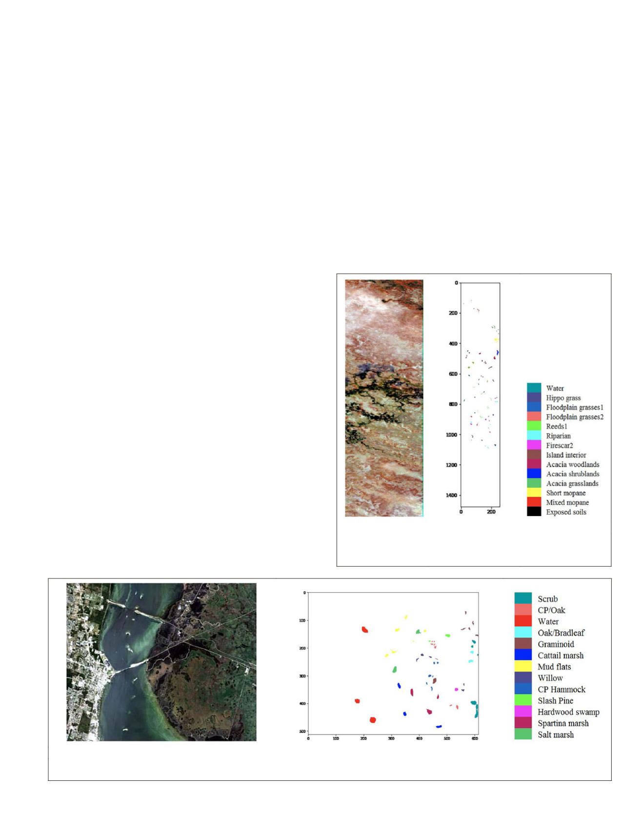
The four widely used hyperspectral data
our experiments. The first data set is Bot
was acquired by the National Aeronautics and Space Admin-
istration (NASA) Earth Observing-1 satellite at 30 m pixel
resolution over the Okavango Delta, Botswana in 2001. It
originally has 242 bands covering the 400–2500 nm portion of
the spectrum in 10 nm windows, but only 145 bands are used
for the analysis after removing the uncalibrated and noisy
bands. This data set contains 14 classes and has a size of 1476
× 256 pixels. A total of 3248 pixels are labeled with the dif-
ferent types of land cover (Neuenschwander
et al.
2005) (see
Figure 2).
The second hyperspectral data set is Kennedy Space
Center (KSC), which was acquired over the Kennedy Space
Center, Florida, on 23March 1996, at a spatial resolution of
18 m. The original data set consists of 220 bands, and it has a
size of 512 × 614 pixels, after removing water absorption and
low signal to noise ratio bands, 176 bands are left. This image
contains 13 classes with a total of 5211 labeled pixels (Ham
et
al.
2005) (see Figure 3).
The third hyperspectral data set is Indian Pines data set.
In June 1992, the NASA Airborne Visible InfraRed Imaging
Spectrometer (AVIRIS) image was acquired over the Indian
Pines agricultural site in northwestern Indiana. AVIRIS is a so-
phisticated optical sensor system including a number of major
subsystems, components, and characteristics. The
AVIRIS
sensor
(b)
(c)
Figure 2. False-color composite image of
BOT
data set and
color map of ground truth. (a) False-color image. (b) Ground
truth. (c) Class legends.
(a)
(b)
(c)
Figure 3. False-color composite image of
KSC
data set and color map of ground truth. (a) False-color image. (b) Ground truth.
(c) Class legends.
PHOTOGRAMMETRIC ENGINEERING & REMOTE SENSING
November 2019
845


