PE&RS November 2019 Full - page 846

receives white light in the
foreoptics, disperses the light
into the spectrum, converts the
photons to electrons, amplifies
the signal, digitizes the signal,
and records the data to high
density tape. This data set con-
tains 145 × 145 pixels, at 20 m
spatial resolution and 10 nm
spectral resolution over the
range of 400–2500 nm. Result-
ing in a 200-band image, twen-
ty noisy and water absorption
bands (104–108, 150–163, and
220) were removed (Jackson
and Landgrebe 2001).
The fourth data set is the
Pavia University. This data set
was acquired by the Reflec-
tive Optics System Imaging
Spectrometer (ROSIS) instrument in 2001, covering the
city of Pavia, Italy (Zhang et al. 2013). The principle and
performance of ROSIS are presented in the following
with emphasis on the sensors, signal conditioning, and
the related data flow. The image scene is centered at the
University of Pavia, with a size of 610 × 340 pixels. After
removing 12 bands due to noise and water absorption,
103 spectral channels remained. This data set contains
nine classes representing the different types of land
cover, and there are 42 776 available samples.
Experimental Settings
In the experiment, we set q1 = q2(W A = W B = 0.5). It means
that nEQB and MCLU usually select the same amount of
samples. When nEQB and MCLU simultaneously select
the same samples, we select informative samples as
supplements from MCLU. Then, these selected samples
are labeled by classifiers. To validate the effectiveness of
the proposed framework, we compare it with four state-
of-the-art hyperspectral image classification methods.
For the Indian Pines data set, we select 12 categories for
classification, and it has 10 062 labeled pixels (the number of
samples more than 100) (see Table 2). Firstly, we randomly
divided the total available data into twoparts for each image:
70% data sets use for training and 30% for testing. And for
the 70% training data, we randomly selected five samples
in each class as the initial labeled data, and then remaining
samples were unlabeled data. In the KSC data set, we ran-
domly divided the total available data into two parts: 50%
for training and 50%for testing. For the 50% training data,
we randomly selectedfive samples in each class as the initial
Table 1. Numbers of samples for the
corresponding classes of the BOT
data set.
Class Name No. Samples
Water 270
Hippo grass 101
Floodplain grasses 1 251
Floodplain grasses 2 215
Reeds1 269
Riparian 269
Firescar 2 259
Island interior 203
Acacia woodlands 314
Acacia shrublands 248
Acacia grasslands 305
Short mopane 181
Mixed mopane 268
Exposed soils 95
Table 2. Numbers of samples for the
corresponding classes of the Indian
Pines data set.
Class Name No. Samples
Corn-no till 1428
Corn-min till 830
Corn 237
Grass/Pasture 483
Grass/Trees 730
Hay-windrowed 478
Soybeans-no till 972
Soybeans-min till 2455
Soybean-clean till 593
Wheats 205
Woods 1265
Building-Grass-Tress-Drives 386
Table 3. Numbers of samples for the
corresponding classes of the KSC
data set.
Class Name No. Samples
Scrub 761
Willow 243
CP Hammock 256
CP/Oak 252
Slash Pine 161
Oak/Broadleaf 229
Water 927
Hardwood swamp 105
Graminiod marsh 431
Spartina marsh 520
Cattail marsh 404
Salt marsh 419
Mud floats 503
(a) (b) (c)
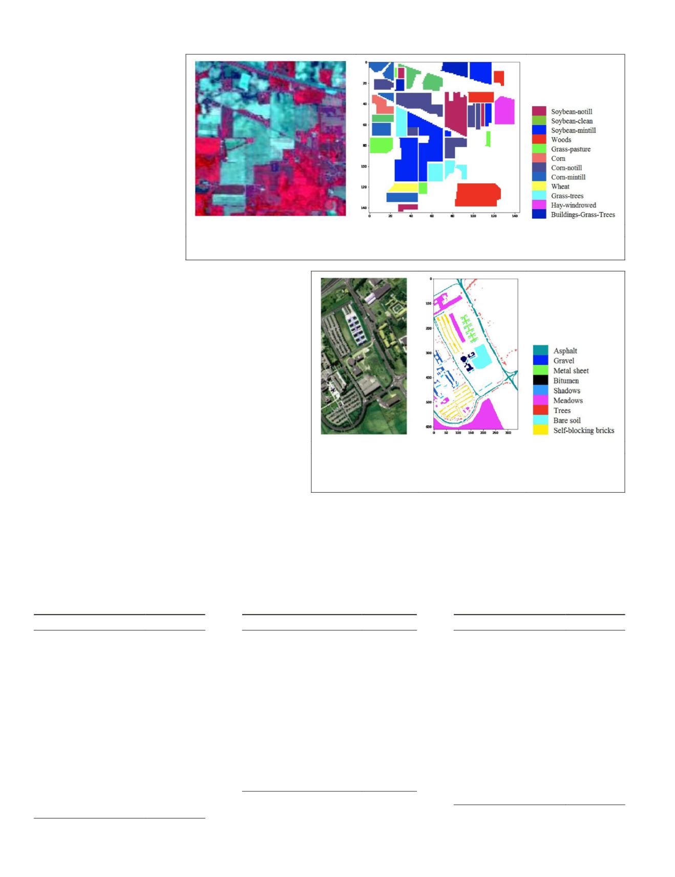
Figure 4. False-color composite image of Indian pines data set and color map of ground
truth. (a) False-color image. (b) Ground truth. (c) Class legends.
(a) (b) (c)
Figure 5. False-color composite image of Pavia university data set
and color map of ground truth. (a) False-color image. (b) Ground
truth. (c) Class legends.
846 November 2019 PHOTOGRAMMETRIC ENGINEERING & REMOTE SENSING