As illustrated in Figure 3, thinning was achieved by super-
imposing a point-grid over the area at a resolution required to
achieve a target pulse density (Table 3). First-returns with the
shortest Cartesian distance to the grid point were selected and
the attributes retained, e.g., selected points were not snapped.
A search window was utilized when selecting points to filter
points that may lie closer to an adjacent grid point (Figure 3),
this was optimized at 2/3 the point-grid resolution to minimize
duplication of returns while maintaining pulse density (Figure
3a). For each first-return selected, the
number of returns
meta-
data value (
X
) was extracted. An additional
X
points with a
corresponding
return number
metadata value were subsequent-
ly selected. For example, if a selected first-return had a
number
of returns
value of Y then [
R
2
,
R
3
,
R
n
, …
R
Y
] additional returns
were selected where the subscript value refers to the
return
number
. Additional returns were again selected by shortest
Cartesian distance from the grid point. Maximum distance for
additional returns was likewise restricted to a search voxel
where the extent (
SW
e
) was determined from an estimate of
canopy height (
z
max
) and an assumed maximum scan angle (
θ
)
of 5° [Equation 1] in Figure 3a. The extracted dataset therefore
simulates a near nadir acquisition with a regular scan pattern
(Baltsavias, 1999), this standardizes simulated capture specifi-
cations aiding comparison between plots and study areas.
SW
e
= 2(
z
max
· tan
θ
)[1].
For the simulated datasets, ground points were identified
and used to compute a Triangulated Irregular Network (
TIN
),
from which height relative to ground was calculated for all re-
turns. Computing a
TIN
and relative height for each simulated
dataset was necessary so that miscalculation of the ground
surface can be accounted for (Magnusson
et al
., 2007).
Identification of ground returns and relative return height
calculation was computed using default settings with the
lasground
and
lasheight
tools respectively from the LAStools
software package, version 130225 (Isenburg, 2012).
A plot with a radius of 11.8 m was clipped from each
thinned and ground normalized dataset to replicate standard
forest inventory plot dimensions (e.g.,
DEWLP
, 2012). Thin-
ning and
TIN
creation were computed for the larger dataset to
ensure all ground returns within the clipped area had a full
neighborhood from which to generate a
TIN
. Furthermore, the
scan pattern towards the edges of the larger dataset became
irregular owing to the circular plot shape; clipping removed
this effect from the smaller plots.
Owing to the density of the original dataset and the sys-
tematic way in which simulated datasets were constructed,
additional realizations could be computed from the original
dataset with minimal duplication of returns between realiza-
tions. Therefore nine simulated datasets were generated for
each plot, where the origin of the sample point grid was offset
recursively by 1/3 of the sampling resolution in both the
x
and
y
direction. From the nine realizations, a robust set of
descriptive statistics were generated and compared to a value
derived from a high pulse density dataset (see below). Gener-
ating different plotwise realizations also allowed the repeat-
ability of
ALS
capture to be assessed (Bater
et al
., 2011).
Metrics
Forest structure could be characterized by three categories
of primary descriptor: (a) canopy height, (b) canopy cover,
and (c) vertical canopy structure (Kane
et al
., 2010; Lefsky
et al
., 2005). With regard to this, three metrics representing
each of these categories were selected: the 95
th
percentile of
non-ground return height as an analogue of dominant canopy
height (Lovell
et al
., 2003); canopy cover was estimated using
1 –
P
gap
(
z
) where
z
equals 1 m; and the coefficient of variation
(
C
v
) of return height as a metric of vertical canopy structure
(Bolton
et al
., 2013; Kane
et al
., 2010; Zimble
et al
., 2003).
Vertically resolved gap probability
P
gap
(
z
) was computed using
ALS
returns weighted by the
return number
, as Armston
et al
.
(2013) concluded this produced a more accurate estimate of
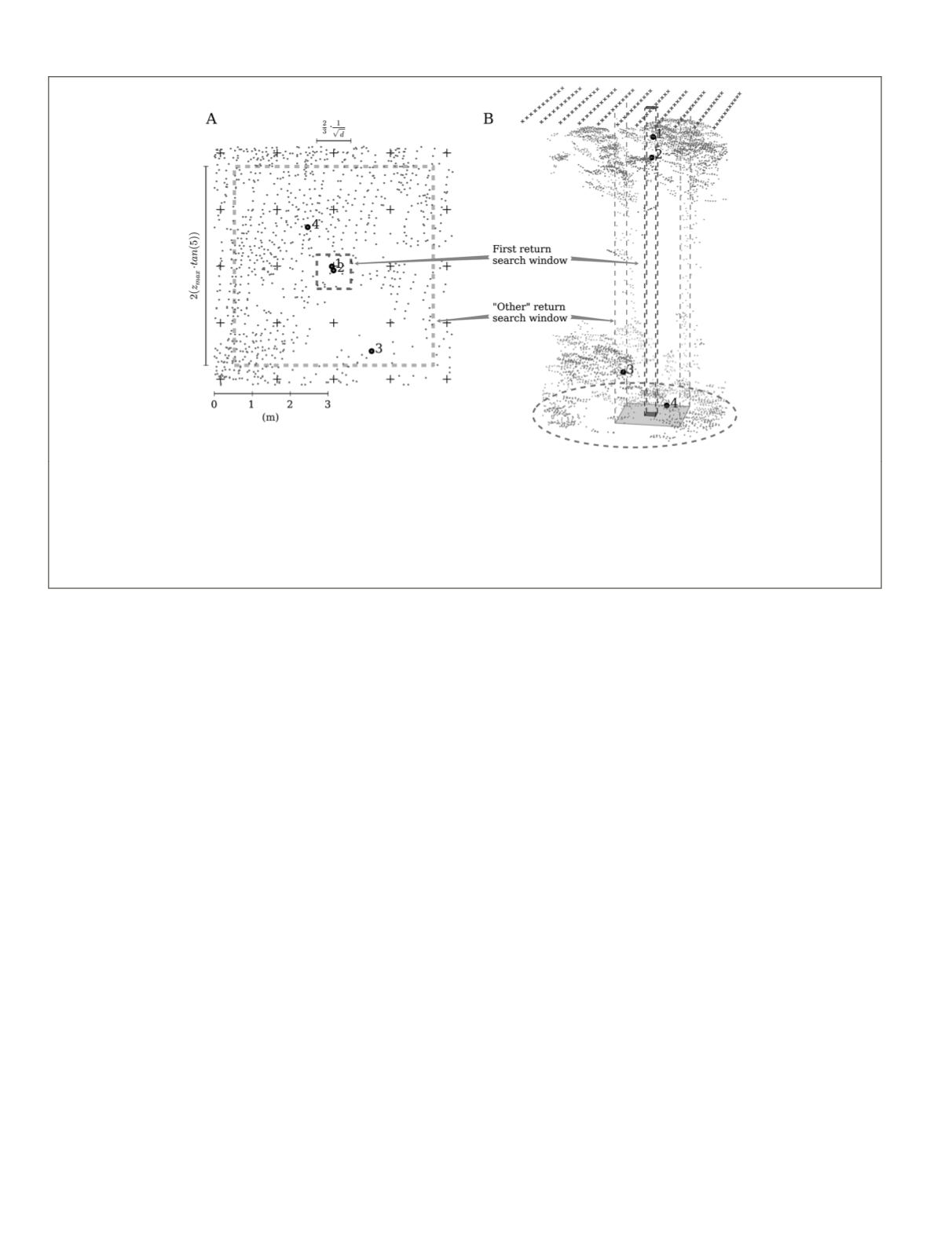
Figure 3. Visualization describing the point cloud thinning technique using a target pulse density of 0.5 pl m
-2
as an example: (A) A single
first return is selected for each grid point (+) where the ALS return with the lowest Cartesian distance is selected. Selection is restricted to
a search-window around each grid point where the search window dimensions are determined by the desired pulse density (
d
). Selection
of
X
further returns, determined by the
number of returns
metadata field (in this case
X
= 4), are again chosen by their proximity to the
grid point. A search-window restricts the maximum distance of “other” returns where the extent is determined by an estimate of the maxi-
mum height of the forest (
z
max
= 40 m) and an assumed scan angle ≤5°, in this way a nadir acquisition is simulated. Nota bene. Points
have been removed from outside the plot boundary to enhance visualization (B), when point clouds were thinned points from outside the
plot boundary could be selected.
628
August 2015
PHOTOGRAMMETRIC ENGINEERING & REMOTE SENSING


