scale factor
λ
is estimated using Equation 22, where (
DD
T
)
ij
refers to the element at the
i
th
row and
j
th
column of the matrix
DD
T
. Equations 23 and 24 are used to estimate the principal
point coordinates (
x
p
,
y
p
) and the principal distance in the Y
direction (
c
y
) is derived from Equation 25. The principal dis-
tance in the X direction (
c
x
) and the non-orthogonality angle
(
α
) are estimated using Equations 26 and 27. Finally, after
estimating the perspective center coordinates (
X
O
,
Y
O
,
Z
O
), the
inverse of the rotation matrix
R
c
w
(i.e.,
R
w
c
) can be derived us-
ing the same procedure previously described.
x
y
L L
L L
L L
L L
L L
L L
X
Y
1
1
2
5
6
9 10
3
4
7
8
11 12
=
Z
L L L
L L L
L L L
X
Y
Z
1
1
2
3
5
6
7
9 10 11
=
+
L
L
L
4
8
12
(18)
x
y
c
c x
c y R
X X
Y Y
Z Z
x
x
p
y
p w
c
o
o
o
1
0
0 0 1
=
− −
−
−
−
−
λ
α
=
−
−
−
=
λ
λ
KR
X X
Y Y
Z Z
KR
X
Y
Z
w
c
o
o
o
w
c
−
λ
KR
X
Y
Z
w
c
o
o
o
(19)
X
Y
Z
L L L
L L L
L L L
L
L
L
0
0
0
1
= −
−
2
3
5
6
7
9 10 11
1
4
8
12
(20)
D KR
L L L
L L L
L L L
c
c x
c y
w
c
x
x
p
y
p
=
=
=
− −
−
λ
λ
α
1
2
3
5
6
7
9 10 11
0
0 0 1
R
w
c
(21)
DD L L L
T
(
)
= + + =
33
9
2
10
2
11
2
2
λ
(22)
DD L L L L L L x
T
p
(
)
= + + =
31
9 1 10 2 11 3
2
λ
(23)
DD L L L L L L y
T
p
(
)
= + + =
32
9 5 10 6 11 7
2
λ
(24)
DD L L L
y c
T
p y
(
)
= + + =
+
(
)
22
5
2
6
2
7
2
2 2 2
λ
(25)
DD L L L L L L
c c x y
T
x y
p p
(
)
= + + =
+
(
)
12
1 5 2 6 3 7
2
λ α
(26)
DD L L L c c x
T
x
x
p
(
)
= + + = +
( )
+
11
1
2
2
2
3
2
2 2
2
2
λ
α
(
)
(27)
The Quaternion-based General Approach
In this section, a quaternion-based approach is proposed to
estimate the
EOP
s regardless of the number or configuration of
available object points. In other words, the quaternion-based
general approach can handle three or more image/object
points in either planar or non-planar configuration. In this
approach, the rotation matrix is iteratively estimated first by
enforcing a simple geometric constraint, and the translation
parameters are estimated afterwards through a linear ap-
proach.
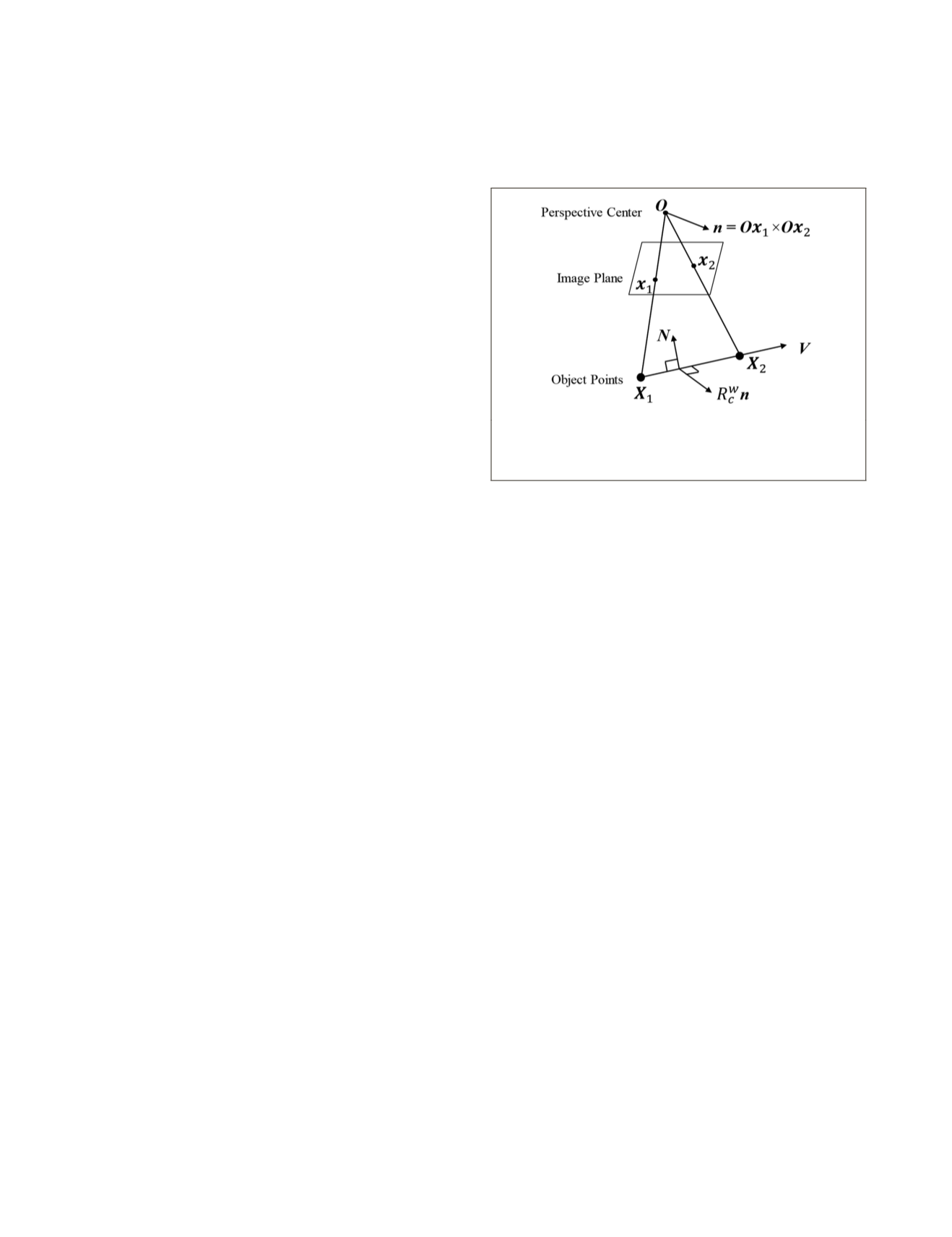
The geometric constraint to derive the rotation starts by
selecting two object points (
X
1
,
X
2
) and their corresponding
image points (
x
1
,
x
2
) from the available points as shown in
Figure 2. The normal vector to the plane encompassing the
perspective center and the image points (
x
1
,
x
2
) is defined as
the cross product of the vectors connecting the perspective
center (
O
) to the image points
x
1
and
x
2
in the image coordi-
nate system, i.e.,
n
=
Ox
1
×
Ox
2
. A vector
N
is then defined in
the
OX
1
X
2
plane and perpendicular to the vector connecting
the two object points (
X
1
,
X
2
), i.e.,
V
=
X
1
–
X
2
. The rotational
relationship between the image and the object coordinate
systems
R
w
c
can be derived by enforcing the cross product
V
×
N
to be aligned along the vector
R
w
c
n
. Figure 2 demonstrates
this geometric constraint.
Figure 2. Geometric constraint to derive the rotation ma-
trix, the cross product
V
×
N
has to be aligned along the
vector
R
w
c
n
.
The above geometric constraint can be expressed mathe-
matically by Equation 28, where
N
i
,
n
i
, and
V
i
are the normal-
ized unit vectors and
e
i
is the misalignment error associated
with the
i
th
point pair derived from the available
n
object
points. To derive the unknown rotation
R
w
c
, least-squares ad-
justment is employed to minimize the Sum of Squared Error
(
SSE
) in Equation 29 for all the possible point pairs selected
from the available
n
points. The number of combinations
to select a point pair out of
n
available points is
n
(
n
− 1)/2,
which will be denoted as
k
. Therefore, the misalignment error
e
i
has to be minimized using all the
k
possible combinations.
e
R
i
i
i
c
w
i
= × −
V N n
(28)
min
R i
k
i
T
i
R i
k
i
i
c
w
i
T
i
i
c
w
i
c
w
c
w
e e
R
R
=
=
∑ ∑
=
× −
(
)
× −
(
)
1
1
min
V N n V N n
=
×
(
)
×
(
)
+ −
(
)
×
=
∑
min
R i
k
i
i
T
i
i
i
T
i
c
w
i
T
i
i
c
w
R
1
2
V N V N n n
n V N
(
)
(29)
In Equation 29, the first two terms are positive constants as
they represent the squared magnitude of the vectors (
V
i
×
N
i
)
and
n
i
, respectively. Therefore to minimize the
SSE
, the rotation
matrix
R
w
c
has to be estimated in a way to maximize the last
term of Equation 29, (
R
w
c
n
i
)
T
(
V
i
×
N
i
). In this term,
n
i
and
V
i
are
directly computed from the image and object point coordi-
nates, and
N
i
depends on the position of the perspective center,
which is unknown. To deal with this dependency without rely-
ing on the perspective center coordinates, the rotation matrix
is derived through an iterative procedure. In the first iteration,
the rotation matrix
R
w
c
is approximated and
N
i
is initially com-
puted as
N
i
=
R
w
c
n
i
×
V
i
. In order to find an approximate esti-
mate for
R
w
c
, the collinearity equations are established for two
points as presented in Equation 30 and the perspective center
coordinates (
X
O
,
Y
O
,
Z
O
) are omitted from those equations by
subtracting the two sets of collinearity equations, which yields
the form in Equation 31. Assuming parallel image space and
object space planes,
λ
1
and
λ
2
will be equivalent and Equation
31 would reduce to the form
X
=
R
w
c
x
as expressed in Equa-
tion 32, where the (
'
) operator indicates the unit vectors along
the involved vectors. This form can be solved for the rotation
matrix
R
w
c
using the introduced quaternion-based procedure
212
March 2015
PHOTOGRAMMETRIC ENGINEERING & REMOTE SENSING


