Procedures to calculate L
λ
for Landsat-7 and ASTER were
taken from Chander
et al
., (2009) and Abrams
et al
. (2002),
respectively.
Surface Temperature (Ts)
At-sensor brightness temperature was calculated using the
following formula (Chander
et al
., 2009):
Ts
K
ln
K
L
=
+
2
1
1
λ
(2)
where
Ts
= Effective at-sensor brightness temperature [K],
K
2
= Calibration constant 2 [K],
K
1 = Calibration constant 1 [W/(m
2
sr μm)],
L
λ
= Spectral
radiance at the sensor᾿s aperture [W/(m
2
sr μm)], and
ln
=
Natural logarithm.
L
λ
for Landsat-7 was calculated using band
ETM6 (10.31-12.36 μm)(Chander
et al
., 2009), and for
ASTER
band TIR4 (10.25-10.95 μm)(Abrams
et al
., 2002).
ASTER NDVI
and
Ts
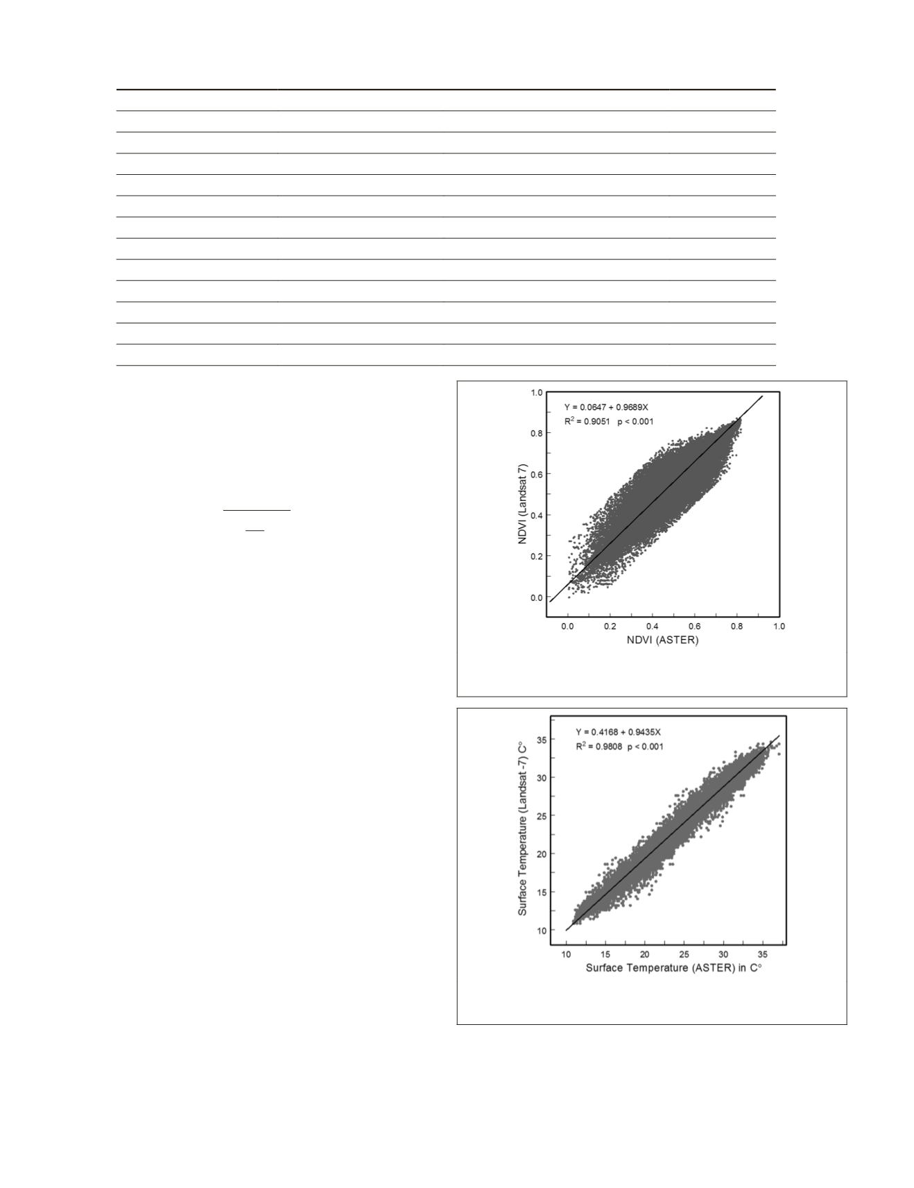
were re-sampled to 30 m resolution using
bilinear interpolation method and adjusted to be comparable
to Landsat equivalents. The adjustment factors were derived
by using linear regression as shown in Figures 2 and 3:
NDVI
Landsat-7
= 0.06 + 0.97
NDVI
ASTER
(3)
(R
2
= 0.905,
p
<0.001)
Ts
Landsat-7
= 0.42 + 0.94Ts
ASTER
(4)
(R
2
= 0.981,
p
<0.001)
Surface-Air Temperature Difference (Ts−Ta)
Surface temperature has long been used for the understand-
ing of vegetation water status (Idso
et al
., 1981). As vegeta-
tion transpires, water loss reduces leaf temperature through
evaporative cooling. In well-watered situations, the vegeta-
tion surface temperature often becomes much lower than
that of the surrounding air. On the other hand water-stressed
vegetation transpire less and vegetation surface temperature
increases, typically rising above the surrounding air tempera-
ture (Jackson, 1982). The difference between the surface and
air temperatures (
Ts−Ta
) is therefore useful to assess vegeta-
tion water status, which has been used in this study.
Half-hourly air temperature data, close to the time of each
satellite overpass, was sourced from the Bureau of Meteorol-
ogy (
and the SILO website
-
dock.qld.gov.au/silo/
) for 13 weather stations across the
region as shown in Plate 1b. The point data of air temperature
(
Ta
) was rasterized, using
inverse distance weighted
(IDW)
method, to match the
Ts
from satellite and to enable the cal-
culation of the surface-air temperature difference (
Ts
−
Ta
).
T
able
1. S
atellite
D
ata
U
sed
in
the
S
tudy
Acquisition Date
Satellite / Sensor
Scene Identification
Sky Condition
04 Sep 2012
Landsat-7
93 / 85
Cloudy in SE
22 Oct 2012
Landsat-7
93 / 85
E & S cloudy
23 Nov 2012
Landsat-7
93 / 85
Partly cloudy
18 Dec 2012
ASTER
AST3A1 1212180020311212190009 Cloud-free
18 Dec 2012
ASTER
AST3A1 1212180020311212190010 Cloud-free
01 Jan 2013
ASTER
AST3A1 1301010032531301070023 Cloud-free
01 Jan 2013
ASTER
AST3A1 1301010032451301070024 Cloud-free
10 Jan 2013
Landsat-7
93 / 85
Cloud-free
26 Jan 2013
Landsat-7
93 / 85
NE cloudy
11 Feb 2013
Landsat-7
93 / 85
Cloud-free
16 Apr 2013
Landsat-7
93 / 85
N & E cloudy
02 May 2013
Landsat-7
93 / 85
Cloud-free
Figure 2. Scatter diagram showing relationship between
ndvi
values from ASTER and Landsat-7.
Figure 3. Scatter diagram showing relationship between tem-
perature values from
aster
and Landsat-7.
232
March 2015
PHOTOGRAMMETRIC ENGINEERING & REMOTE SENSING


