a grid-based representation, and (c) it defines neighborhood
relations of the generated voxels as well as the points within
them. It is noteworthy that selecting the size of voxels is a
trade-off between the efficiency of processing and the preser-
vation of details. Generally speaking, the smaller the voxels,
the more details will be retained. In this work, the size of
voxels is determined empirically according to the demands
of the application. For example, in our experiments, for the
reconstruction of major building elements (e.g., facades and
roofs) the size of voxel was set to 0.2 m, but in other cases, it
would depend on the requirements of the application.
Calculation of Geometric Cues
Geometric cues represent the relation between two voxels.
The calculation of these cues includes two major steps: the
estimation of voxel attributes and the application of percep-
tual grouping laws.
Estimation of Voxel Attributes
The attributes of a voxel
V
describe the geometric character-
istics of points inside
V
, including three groups of features:
spatial positions, geometric features, and normal vectors cal-
culated from points. The spatial position stands for the spatial
coordinate of the centroid
X
of points within a voxel
V
. The
geometric features are eigenvalue based features (Weinmann
et al.
, 2015) related to the 3D distribution of points inside
a voxel. In particular, we apply four local shape features,
namely the linearity
Le
, the planarity
Pe
, the scattering
Se
,
and the change of curvature Ce (Weinmann
et al.
, 2015).
These four features are calculated from eigenvalues
e
1
≥
e
2
≥
e
3
≥
0 by eigenvalue decomposition (
EVD
) of the 3D structure
tensor (i.e., covariance matrix), which is computed from 3D
coordinates of all points inside the voxel.
As described in Weinmann
et al.
(2015),
Le
,
Pe
, and
Se
re-
late to 1D, 2D, and 3D structures of points, respectively, while
Ce
captures the curvature of the surface formed by points.
The normal vector
N
of points within
V
is obtained from the
eigenvectors of the aforementioned tensor. Since noise and
outliers are always a problem, the estimation of eigenvalues
and eigenvectors is susceptible to errors in the coordinates of
points. To alleviate this problem, we use the weighted covari-
ance matrix proposed in (Salti
et al.
, 2014), assigning smaller
weights to points who are distant from the centroid. The
covariance matrix M is calculated as follows:
M
r d
r d p X p X
i
i d r
i d r
i
i
i
T
i
i
=
−
(
)
−
−
−
≤
≤
∑
∑
1
:
:
__
__
(
)(
)(
)
(1)
where
p
i
denotes the point in the support region of size
r
for
normal vector calculation. The size
r
of the
3
2
d
y
support
region equals to
d
v
, where
d
v
is the size of the voxel.
X
– is the
centroid of the points. Here,
d
i
stands for the distance of
p
i
from the centroid.
Geometric Cues Using Perceptual Grouping Laws
To measure the proximity of the voxels
V
i
and
V
j
, the Euclid-
ean distance
D
p
ij
= |
X
i
−
X
j
| between the centroids
X
i
and
X
j
of
V
i
and
V
j
are used. As far as the second perceptual group-
ing criterion, similarity, is concerned, it is assumed that the
similarity of the spatial distributions of points inside a pair of
voxels is reflected by the similarity of their geometric fea-
ture values. The similarity measure
D
s
ij
between
V
i
and
V
j
in
the four dimensional space of the features defined earlier is
calculated by the histogram intersection kernel (Papon
et al.
,
2013). The third perceptual grouping criterion, continuity, is
evaluated based on the smoothness (Awrangjeb and Fraser,
2014) and the convexity (Stein
et al.
, 2014) of the surface
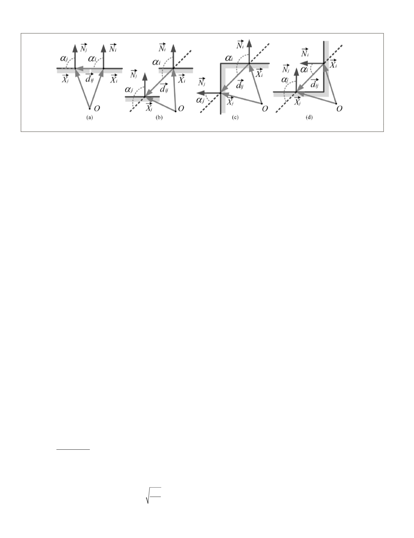
formed by the points inside adjacent voxels. Here, we make
an assumption that the connection types between voxels are
mainly as follows: smooth, “stair-like”, convex, and concave.
Sketches of these four types of connections are shown in Fig-
ure 3. The smoothness
D
m
ij
is related to the difference of angles
between normal vectors
N
i
and
N
j
. The convexity
D
o
ij
depends
on the local configuration of the surfaces formed by points of
two adjacent voxels. A pair of surface patches is considered
to be highly connective if the local configuration is convex.
Whether the local configuration is defined as convex or con-
cave is related to the relation of
N
i
and
N
j
and the vector
d
ij
joining the centroids
X
i
and
X
j
, where
d
ij
= (
X
j
−
X
i
)/|
X
i
–
X
j
|.
As illustrated in Figure 3, angles α
i
and α
j
are calculated. Here,
α
represents the angle between the normal vector
N
and the
vector
d
ij
. If
α
i
−
α
j
>
θ
, the surface connectivity is defined as
a convex connection, where
θ
is the threshold for judging
convexity. Otherwise, it is considered a concave connection.
Here,
θ
is calculated by a sigmoid function determined by the
difference of
α
i
and
α
j
, according to the description in (Stein
et al.
, 2014). The surface continuity
D
c
ij
is a combination of
the smoothness
D
m
ij
and the convexity
D
o
ij
, which is calculated
according to Equation 2, signing a higher degree-of-proximity
to gradual convex or smooth connected surfaces. For both
convex/non-convex situations, the first term of Equation 2
is related to the measure of smoothness
D
m
ij
= (
α
i
−
α
j
)
2
, which
is approximated by the difference between angles
α
i
and
α
j
instead of using the angle between normal vectors
N
i
and
N
j
. The second term in Equation 2 is associated with the
measure of convexity
D
o
ij
, which is different in the two cases.
In the convex case, the measure of convexity is defined as
D
o
ij
= (
π
−
α
i
−
α
j
). In the concave case, the measure of convex-
ity is defined by a constant penalty, namely
D
o
ij
=
π
2
. Accord-
ing to Equation 2, a high degree of continuity (a low value of
D
c
ij
) is assigned to pairs of surfaces that are classified as being
convex, ”stair-like”, or smooth (indicated by
α
i
−
α
j
≤
θ
), if the
corresponding angular difference is small.
Figure 3. Local configurations of surfaces: (a) smooth, (b) “stair-like”, (b) convex, and (c) concave connections.
380
June 2018
PHOTOGRAMMETRIC ENGINEERING & REMOTE SENSING


