summed, and then divided by 74. Figure 9b
shows the spatial gradient (forward differ-
ence) of the pixel profiles, with the value of
a pixel subtracted from the adjacent pixel,
squared, summed, and then divided by 74.
For all three of these metrics,
EV
-1 and
EV
-1.3 appear to have the strongest signal, where higher values
are ideal, as they indicate a greater degree of detection of
detected change across the cracks. The anomalous drop in the
value of
EV
0 is likely due to lower image acuity for one of the
images in the image pair, while the cause of the acuity loss is
uncertain. Even so, a clear trend in the relationship between
EV
setting and crack detection is observable in Figures 9a and 9b.
As shown in Figure 10, the signal and noise
RMSD
values
tend to co-vary with the
EV
bias values. The signal
RMSD
however, exhibits a trend with EVs −1.7 to −1 exhibiting the
highest signal, and some of the higher
SNR
scores, suggest-
ing that this narrow range of
EV
biases is preferable for crack
detection. Visually, within the change detection images and
pixel profiles, cracks the equivalent width of a single pixel of
GSD
are readily identifiable as change objects in most of the
image pairs (Figure 8d).
Discussion and Conclusion
This goal of this study is to determine how to optimize
radiometric parameters of
DSLR
cameras to enable reliable
image-based change detection, through the exploration
of three research questions: (1) with what combination of
exposure settings can the dynamic range of image brightness
values be maximized, while achieving high image acuity?; (2)
what is the characteristic spatial trend in brightness response
within image frames, how do these trends vary with differ-
ent exposure parameters, and how well can within image
trends be balanced or normalized?; and (3) how can between
image differences in radiometric brightness response due
to noise be minimized and due to signal be maximized for
multi-temporal
RSI
pairs, by proper selection of exposure
parameters? These questions were tested and analyzed within
an experimental framework that analyzed the influence of five
variables,
EV
,
WB
, light metering,
ISO
, and relative aperture, on
Table 3.
EV
bias +/- 0 images from four
collection dates, at two times per day,
of two different scenes, using two light
metering modes.
APEX EV Count
Percentage of Category
13.7
1
1%
14.3
32
17%
14.7
110
59%
15
40
21%
15.3
3
2%
15.7
1
1%
All
187
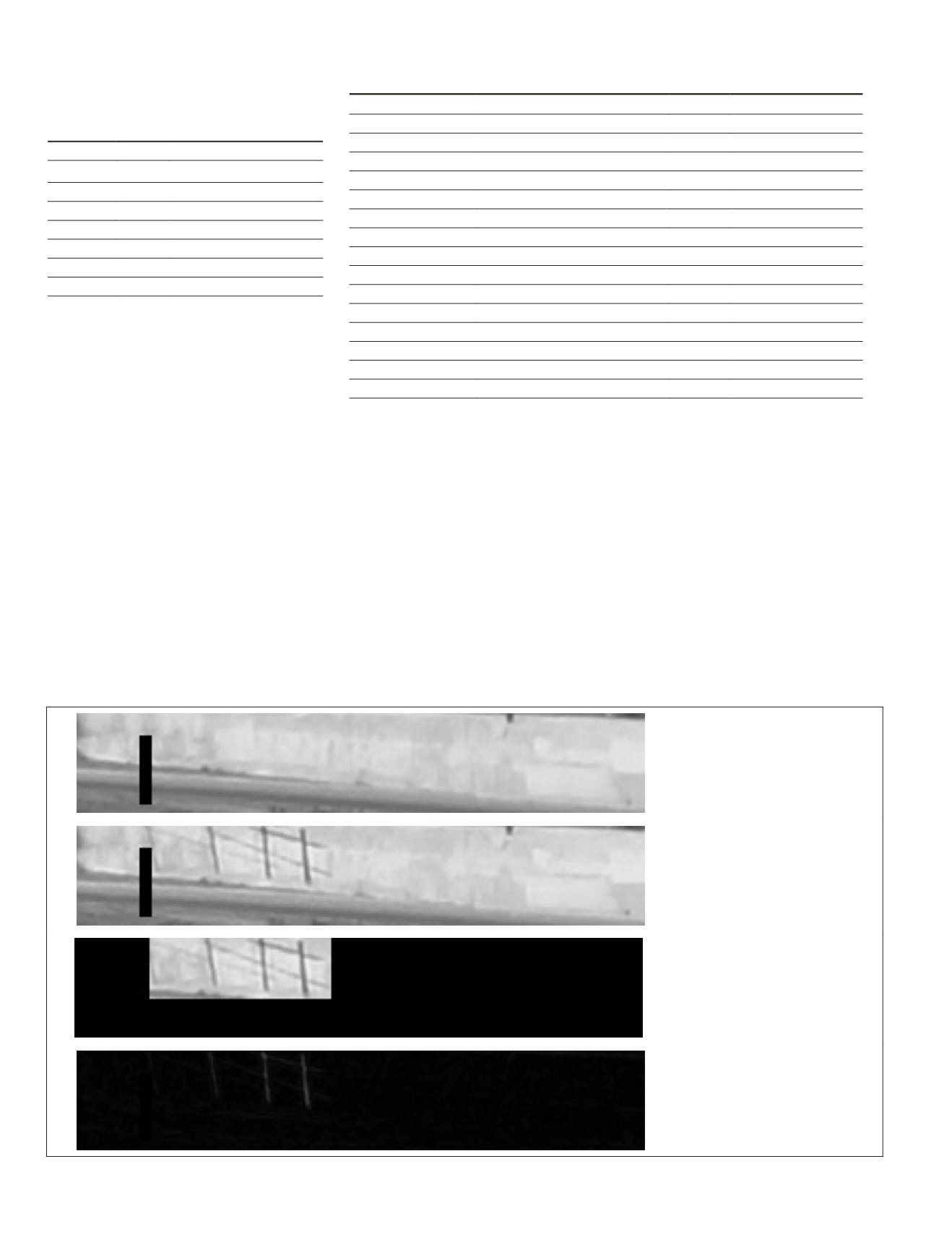
(a)
Figure 8: (a) Subset of oblique
intensity image used for
simulated crack detection
experiment “before” (time −1)
image of a concrete wall (with
black rectangular mask over a
foreground object) difference;
(b) Subset of oblique intensity
image used for simulated crack
detection experiment “after”
(time−2) image containing black
tape segments representing
cracks of varying widths; ( c)
Subset of oblique intensity
image used for simulated crack
detection experiment “after”
image subset for the bounding
rectangle encompassing
simulated cracks (“signal
subset”) and other area (“noise
subset”) masked in black; and
(d) Subset of oblique intensity
image used for simulated crack
detection experiment difference
image of the “signal subset.”
(b)
(c)
(d)
Table 4. The
APEX
offsets by metering mode, relative to the target
EV
value of 14.7.
APEX EV Offset
Metering Mode
Count Percent of mode
-0.6
Center-weighted average
1
2%
-0.3
Center-weighted average
2
4%
0
Center-weighted average
40
71%
+0.3
Center-weighted average
12
21%
+1.3
Center-weighted average
1
2%
-1
Multi-segment
1
0%
-0.6
Multi-segment
11
2%
-0.3
Multi-segment
125
20%
0
Multi-segment
329
52%
+0.3
Multi-segment
139
22%
+0.6
Multi-segment
18
3%
+1
Multi-segment
5
1%
+1.3
Multi-segment
1
0%
Total
Center-weighted average
56
Total
Multi-segment
629
156
March 2018
PHOTOGRAMMETRIC ENGINEERING & REMOTE SENSING


