disparity map with dataset 65246. However, the results seem
different with the other dataset, e.g., the
JR
result shown in
the last column of Figure 8b looks overly smoothed and its
density is more incomplete than the other two (but this does
not mean it is sparse). Please also note that both disparity
maps from
JPL
(see the second column of Figure 8) contains a
few spikes which are removed for visualization.
Given the error bounds calculated from the manual mea-
surements, the matching scores and rewarding scores of each
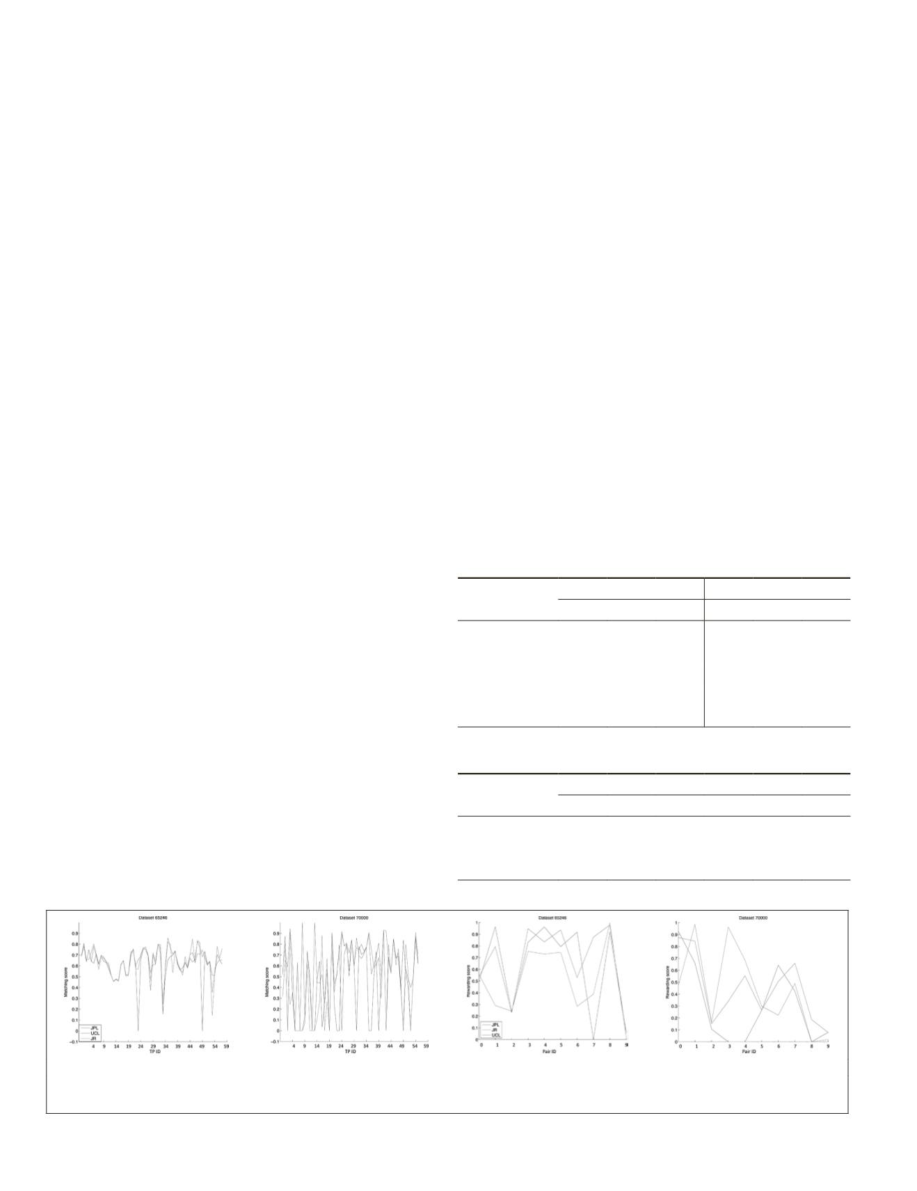
tie-point are evaluated and the results are shown in Figure
9. Matching scores of three algorithms are generally similar
when they can define a tie-point, but when it fails to define a
tie-point no score was awarded, e.g., see
JPL
matching scores
of
ID
23 and 49 in Figure 9a. The rewarding score of
UCL
’s
disparity map is generally lower than the other two with the
dataset 65246 (See Figure 9c). However, it is improved with
the other dataset having more depth discontinuities.
The total scores were calculated using an equal weight of the
matching scores and rewarding scores, and the results are sum-
marized in Table 2, where the best scores for certain datasets are
labeled in bold font. We can observe that for dataset 65246 that
JR
’s stereo matching pipeline produced the best result for the
overall area. To understand this result clearly, it is worth men-
tioning that the total score (
TS
) shown in (Equation 8) has been
designed to award more scores if a disparity map defines all
queried tie-points; in other words, no score is given if there is no
corresponding tie-point in a disparity map. Thus, this metric is
generally favored for a dense and smooth disparity map, which
we believe why
JR
’s results perform best on both test datasets.
To give more weight on the accuracy of an algorithm,
we modified Equation 8 not to penalize when they failed to
define a queried tie-point in a disparity map, and called this
score,
TS-B
. The results of
TS-B
of both datasets are also pre-
sented in Table 3.
We also introduce a new term
MFR
representing the Match-
ing Failure Rate.
MFR
can be used as an indicator for either the
incompleteness of a disparity map or how conservative the
algorithm is. As shown in Table 2,
JPL
’s results have higher
MFR
,
but without counting on the match failure area (i.e., using
TS-B
)
JPL
’s pipeline produced the best result on the dataset 65246. For
dataset 70000,
JPL
’s pipeline gets the second best score while
UCL
’s processing pipeline has produced the best accuracy.
Discussion and Conclusions
In this paper, we introduced an accuracy evaluation method
to assess the stereo matching results. The main motivation of
this work is to provide a straightforward method which can
be applied to the stereo matching evaluation work of plane-
tary rover missions, where it is currently impossible to obtain
ground truth data.
We have demonstrated the use of a generic portable stereo
workstation including a stereo cursor from the open source
StereoWS tool to produce visually correct tie-points of a stereo
pair, i.e., manual tie-points, with the help of a softcopy stereo
display. The manual tie-points from stereo measurements are
not identical for all candidate tie-points, but our assumption
is that the variation of multiple measurements can be used to
estimate the confidence of a tie-point, and these confidence
values can quantitatively evaluate the quality of disparity
maps from different algorithms. Based on this idea, we have
defined useful evaluation metrics using the statistics of mul-
tiple measurements (such as means and variance). We also de-
fine three types of tie-points to test the performance at highly
textured region, textureless region, and occluded region. The
performance of textureless region is quite interesting for
DTM
construction from orbital imagery but this is left for the future
work. Type (b) tie-points are related to the scene occlusion. At
the moment, we populate these points manually but it is also
possible to design a semi-automatic pipeline to collect these
points, e.g., detect one tie-point by conventional feature detec-
tor and find adjacent feature from background manually.
It is worth noting that in these experiments, the number
of tie-points, particularly for the discontinuities, may not be
sufficient in some cases. It would have been better to add
more tie-points. However, we erred on the side of setting
an experiment which could be accomplished with a group
of ten “citizen scientists” within a limited time period (one
week). Other comparison results, e.g., disparity density or 3D
accuracy, could also be employed in future experiments to
improve the final matching score.
During the evaluation work, we implemented an open
source stereo workstation with an integrated stereo matching
method that is used to produce the
UCL
results shown in the
evaluation. We have published the Java code of the Stereo
(a)
(b)
(c)
(d)
Figure 9. (a) Individual matching scores of the processing results of two datasets; and (b) Rewarding scores from 10 tie-point
pairs in two datasets.
Table 2. Total score (
TS
) estimated from (8) with
α
= 0.5.
Dataset
65246
70000
UCL
JPL JR
UCL
JPL
JR
Matching score 63.96 61.26 64.16 50.45 45.15 57.01
MFR(%)
0.00 3.50 0.00 16.10 26.80 10.70
Rewarding score 50.11 61.87 67.15 43.07 31.05 44.64
MFR(%)
0.00 10.00 0.00 10.00 30.00 0.00
TS
55.65 61.63 65.95 46.02 36.69 49.59
Table 3. Total Score B (TS-B) which is similar to
TS
but
removes the effect of missing tie-points.
Dataset
65246
70000
UCL
JPL JR
UCL
JPL
JR
Matching score 63.96 63.45 64.16 60.11 61.67 63.86
Rewarding score 50.11 68.75 67.15 47.85 44.35 44.64
TS-B
55.65 66.63 65.95 52.75 51.28 52.33
166
March 2018
PHOTOGRAMMETRIC ENGINEERING & REMOTE SENSING


