in 3D, i.e., Participants 5 and 6 (see Figure7c]. These outliers
were then removed before calculating the error bounds.
Figure 7a, 7c, and 7e summarize the errors from the inlier
means
d
(
t
k
i
,
m
k
i
) of all tie-points from 9 participants. It is
observed that tie-points from the indistinctive textures are
generally difficult to select, for example,
t
a
1
,
t
a
4
,
t
a
5
,
t
a
7
, and
t
a
9
in
the feature based tie-points have larger measurement varia-
tion and more outliers [see Fig. 7(b)]. This reconfirms our
understanding that a stereo visualization can help us detect
correct tie-points better around the object boundary than
within plain/repetitive texture.
One interesting observation from the error graph is that
the performance of participant 5, who consistently produced
a large measurement error regardless of the type of dataset,
deteriorates when a tie-point is closer to a camera (i.e., a
larger disparity). For example, the measurement errors for
t
a
3
,
t
a
7
,
t
a
11
, and
t
a
15
(which is the bottom row of the grid in Figure
5b) are getting worse than the rest, and we can see this pattern
in Figure 7c.
The error metrics of measurements are evaluated and sum-
marized in Table 1. Without the removal of outliers, the total
measurement error increases significantly. The maximum of
was recorded with the feature based tie-points (20.83), where-
as the minimum (8.39) was obtained from the discontinuity
tie-points. However, after removing obvious outliers (i.e.,
δ
>10 in Equation 2), the measurement errors drop sharply to
less than two pixels with small standard variation (see
e
in
and
avg.
σ
x
in Table 1). As mentioned earlier, we believe this hap-
pens because of the outliers introduced by a few participants
who fuse a stereo pair differently than the rest.
Table 1. Measurement errors of C33 (
N.B.
Type (a) results
of participant 2 was excluded due to the incomplete of
measurements.)
Type
e
tot
e
in
e
out
avg.
σ
x
a
20.83
1.61
40.04
0.92
b
10.83
1.10
22.98
1.71
c
8.39
1.78
16.65
0.93
avg.
13.35
1.50
26.56
1.19
The bar charts of the inlier measurements for three datasets
are shown in the second column of Figure 7. Each bar chart
summarizes the differences between the inlier measurements
and the mean of the inlier measurements. Type (b) tie-point
selection appears to be more difficult as participants are
often required to fuse the stereo cursor around textureless
or smooth (i.e., small depth separation) areas. As a conse-
quence, the inlier measurements of regular grid tie-points
are generally inconsistent (i.e., avg.
σ
x
= 1.71 ) compared to
the others (see Figure 7d). On the other hand, strong depth
discontinuity around an object boundary from Type (c) tie-
points improve the consistency of
the measurements (see Figure 7f).
We have found that the maximum
standard deviation is 2.56 pixels,
the minimum standard deviation is
0.37 pixels, and the average is 0.93
pixels.
It is also interesting to see that
SIFT
keypoints performs the best for
stereo fusion. Its average standard
deviation is 0.92 which is margin-
ally better than the second best
but the left tie-points of Type (a)
were selected simply based on the
texture information (see Figure 7b).
We think that the distinctive gradi-
ent information around a keypoint
can improve the performance of
stereo measurements.
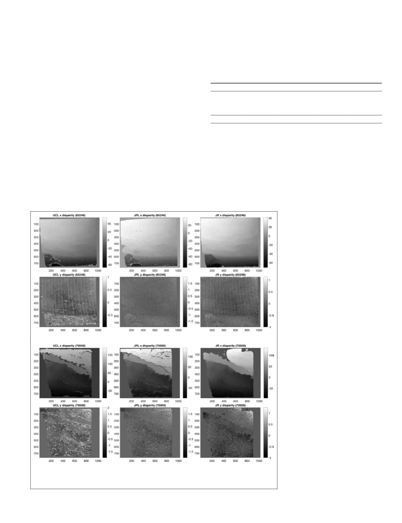
Results of Automated Stereo Matching
In our evaluation, we have col-
lected two sets of processing
results (i.e., a and disparity map)
from
UCL
,
JPL
, and
JR
. Figure 8a and
8b, respectively, represent these
disparity maps of dataset 65246
and 70000 from ExoMars PanCam
Test Campaign, and each column
of the figure represents the results
from different organisations. To our
best knowledge all three algorithms
have been developed based on a
variation of a correlation-based
stereo matching algorithm with
an adaptive least square fitting
technique (Deen and Lorre, 2005;
Otto and Chau, 1989), but all
results seem to be slightly different
in terms of the completeness and
the estimated values of a dispar-
ity map. All three results were
able to produce a relatively denser
(a)
(b)
Figure 8. Example of disparity maps: (a) x and y disparity maps of dataset 65246; (b) and
dataset 70000;
UCL
,
JPL
, and
JR
results are shown in the first, the second and the last column.
PHOTOGRAMMETRIC ENGINEERING & REMOTE SENSING
March 2018
165


